1. Deep Learning with PyTorch

A Gentle Introduction to `torch.autograd`

torch.autograd is PyTorch’s automatic differentiation engine that powers neural network training. In this section, you will get a conceptual understanding of how autograd helps a neural network train.

Background

Neural networks (NNs) are a collection of nested functions that are executed on some input data. These functions are defined by parameters (consisting of weights and biases), which in PyTorch are stored in tensors.

Training a NN happens in two steps:

Forward Propagation: In forward prop, the NN makes its best guess about the correct output. It runs the input data through each of its functions to make this guess.

Backward Propagation: In backprop, the NN adjusts its parameters proportionate to the error in its guess. It does this by traversing backwards from the output, collecting the derivatives of the error with respect to the parameters of the functions (gradients), and optimizing the parameters using gradient descent.

Usage in PyTorch

Let’s take a look at a single training step. For this example, we load a pretrained resnet18 model from torchvision. We create a random data tensor to represent a single image with 3 channels, and height & width of 64, and its corresponding label initialized to some random values. Label in pretrained models has shape (1,1000).

Note

This tutorial work only on CPU and will not work on GPU (even if tensor are moved to CUDA).

CodeOut

import torch
from torchvision.models import resnet18, ResNet18_Weights
model = resnet18(weights=ResNet18_Weights.DEFAULT)
data = torch.rand(1, 3, 64, 64)
labels = torch.rand(1, 1000)

Downloading: "https://download.pytorch.org/models/resnet18-f37072fd.pth" to /var/lib/jenkins/.cache/torch/hub/checkpoints/resnet18-f37072fd.pth

  0%|          | 0.00/44.7M [00:00<?, ?B/s]
  6%|5         | 2.53M/44.7M [00:00<00:01, 26.4MB/s]
 11%|#1        | 5.05M/44.7M [00:00<00:01, 25.0MB/s]
 31%|###1      | 14.1M/44.7M [00:00<00:00, 53.7MB/s]
 66%|######5   | 29.4M/44.7M [00:00<00:00, 94.3MB/s]
100%|##########| 44.7M/44.7M [00:00<00:00, 93.1MB/s]

Next, we run the input data through the model through each of its layers to make a prediction. This is the forward pass.

prediction = model(data) # forward pass

We use the model’s prediction and the corresponding label to calculate the error (loss). The next step is to backpropagate this error through the network. Backward propagation is kicked off when we call .backward() on the error tensor. Autograd then calculates and stores the gradients for each model parameter in the parameter’s .grad attribute.

loss = (prediction - labels).sum()
loss.backward() # backward pass

Next, we load an optimizer, in this case SGD with a learning rate of 0.01 and momentum of 0.9. We register all the parameters of the model in the optimizer.

optim = torch.optim.SGD(model.parameters(), lr=1e-2, momentum=0.9)

Finally, we call .step() to initiate gradient descent. The optimizer adjusts each parameter by its gradient stored in .grad.

optim.step() #gradient descent

At this point, you have everything you need to train your neural network. The below sections detail the workings of autograd - feel free to skip them.

Differentiation in Autograd

Let’s take a look at how autograd collects gradients. We create two tensors a and b with requires_grad=True. This signals to autograd that every operation on them should be tracked.

import torch

a = torch.tensor([2., 3.], requires_grad=True)
b = torch.tensor([6., 4.], requires_grad=True)

We create another tensor Q from a and b.

\[ Q = 3a^3 - b^2 \]

Q = 3*a**3 - b**2

Let’s assume a and b to be parameters of an NN, and Q to be the error. In NN training, we want gradients of the error with respect to parameters, i.e.

\[ \frac{\partial Q}{\partial a} = 9a^2 \]

\[ \frac{\partial Q}{\partial b} = -2b \]

When we call .backward() on Q, autograd calculates these gradients and stores them in the respective tensors’ .grad attribute.

We need to explicitly pass a gradient argument in Q.backward() because it is a vector. gradient is a tensor of the same shape as Q, and it represents the gradient of Q with respect to itself, i.e.

\[ \frac{dQ}{dQ} = 1 \]

Equivalently, we can also aggregate Q into a scalar and call backward implicitly, like Q.sum().backward().

external_grad = torch.tensor([1., 1.])
Q.backward(gradient=external_grad)

Gradients are now deposited in a.grad and b.grad.

CodeOut

# check if collected gradients are correct
print(9*a**2 == a.grad)
print(-2*b == b.grad)

tensor([True, True])
tensor([True, True])

Optional Reading - Vector Calculus using `autograd`

Mathematically, if you have a vector valued function $\vec{y}=f(\vec{x})$, then the gradient of $\vec{y}$ with respect to $\vec{x}$ is a Jacobian matrix $J$:

\[ J = \left(\begin{array}{cc} \frac{\partial \bf{y}}{\partial x_{1}} & ... & \frac{\partial \bf{y}}{\partial x_{n}} \end{array}\right) = \left(\begin{array}{ccc} \frac{\partial y_{1}}{\partial x_{1}} & \cdots & \frac{\partial y_{1}}{\partial x_{n}}\\ \vdots & \ddots & \vdots\\ \frac{\partial y_{m}}{\partial x_{1}} & \cdots & \frac{\partial y_{m}}{\partial x_{n}} \end{array}\right) \]

Generally speaking, torch.autograd is an engine for computing vector-Jacobian product. That is, given any vector $\vec{v}$, compute the product $J^{T}\cdot \vec{v}$.

If $\vec{v}$ happens to be the gradient of a scalar function $l=g\left(\vec{y}\right)$:

\[ \vec{v} = \left(\begin{array}{ccc}\frac{\partial l}{\partial y_{1}} & \cdots & \frac{\partial l}{\partial y_{m}}\end{array}\right)^{T} \]

then by the chain rule, the vector-Jacobian product would be the gradient of $l$ with respect to $\vec{x}$:

\[ J^{T}\cdot \vec{v}=\left(\begin{array}{ccc} \frac{\partial y_{1}}{\partial x_{1}} & \cdots & \frac{\partial y_{m}}{\partial x_{1}}\\ \vdots & \ddots & \vdots\\ \frac{\partial y_{1}}{\partial x_{n}} & \cdots & \frac{\partial y_{m}}{\partial x_{n}} \end{array}\right)\left(\begin{array}{c} \frac{\partial l}{\partial y_{1}}\\ \vdots\\ \frac{\partial l}{\partial y_{m}} \end{array}\right)=\left(\begin{array}{c} \frac{\partial l}{\partial x_{1}}\\ \vdots\\ \frac{\partial l}{\partial x_{n}} \end{array}\right) \]

This characteristic of vector-Jacobian product is what we use in the above example; external_grad represents $\vec{v}$.

Computational Graph

Conceptually, autograd keeps a record of data (tensors) & all executed operations (along with the resulting new tensors) in a directed acyclic graph (DAG) consisting of Function objects. In this DAG, leaves are the input tensors, roots are the output tensors. By tracing this graph from roots to leaves, you can automatically compute the gradients using the chain rule.

In a forward pass, autograd does two things simultaneously:

run the requested operation to compute a resulting tensor, and
maintain the operation’s gradient function in the DAG.

The backward pass kicks off when .backward() is called on the DAG root. autograd then:

computes the gradients from each .grad_fn,
accumulates them in the respective tensor’s .grad attribute, and
using the chain rule, propagates all the way to the leaf tensors.

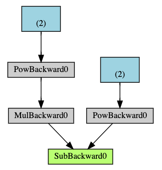
Below is a visual representation of the DAG in our example. In the graph, the arrows are in the direction of the forward pass. The nodes represent the backward functions of each operation in the forward pass. The leaf nodes in blue represent our leaf tensors a and b.

Note

DAGs are dynamic in PyTorch. An important thing to note is that the graph is recreated from scratch; after each .backward() call, autograd starts populating a new graph. This is exactly what allows you to use control flow statements in your model; you can change the shape, size and operations at every iteration if needed.

Exclusion from the DAG

torch.autograd tracks operations on all tensors which have their requires_grad flag set to True. For tensors that don’t require gradients, setting this attribute to False excludes it from the gradient computation DAG.

The output tensor of an operation will require gradients even if only a single input tensor has requires_grad=True.

CodeOut

x = torch.rand(5, 5)
y = torch.rand(5, 5)
z = torch.rand((5, 5), requires_grad=True)

a = x + y
print(f"Does `a` require gradients? : {a.requires_grad}")
b = x + z
print(f"Does `b` require gradients?: {b.requires_grad}")

Does `a` require gradients? : False
Does `b` require gradients?: True

In a NN, parameters that don’t compute gradients are usually called frozen parameters. It is useful to “freeze” part of your model if you know in advance that you won’t need the gradients of those parameters (this offers some performance benefits by reducing autograd computations).

Another common usecase where exclusion from the DAG is important is for finetuning a pretrained network.

In finetuning, we freeze most of the model and typically only modify the classifier layers to make predictions on new labels. Let’s walk through a small example to demonstrate this. As before, we load a pretrained resnet18 model, and freeze all the parameters.

from torch import nn, optim

model = resnet18(weights=ResNet18_Weights.DEFAULT)

# Freeze all the parameters in the network
for param in model.parameters():
    param.requires_grad = False

Let’s say we want to finetune the model on a new dataset with 10 labels. In resnet, the classifier is the last linear layer model.fc. We can simply replace it with a new linear layer (unfrozen by default) that acts as our classifier.

model.fc = nn.Linear(512, 10)

Now all parameters in the model, except the parameters of model.fc, are frozen. The only parameters that compute gradients are the weights and bias of model.fc.

# Optimize only the classifier
optimizer = optim.SGD(model.parameters(), lr=1e-2, momentum=0.9)

Notice although we register all the parameters in the optimizer, the only parameters that are computing gradients (and hence updated in gradient descent) are the weights and bias of the classifier.

The same exclusionary functionality is available as a context manager in torch.no_grad().

Neural Networks

Neural networks can be constructed using the torch.nn package.

Now that you had a glimpse of autograd, nn depends on autograd to define models and differentiate them. An nn.Module contains layers, and a method forward(input) that returns the output.

For example, look at this network that classifies digit images:

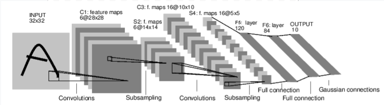
It is a simple feed-forward network. It takes the input, feeds it through several layers one after the other, and then finally gives the output.

A typical training procedure for a neural network is as follows:

Define the neural network that has some learnable parameters (or weights)
Iterate over a dataset of inputs
Process input through the network
Compute the loss (how far is the output from being correct)
Propagate gradients back into the network’s parameters
Update the weights of the network, typically using a simple update rule: weight = weight - learning_rate * gradient

Define the network

Let’s define this network:

CodeOut

import torch
import torch.nn as nn
import torch.nn.functional as F


class Net(nn.Module):

    def __init__(self):
        super(Net, self).__init__()
        # 1 input image channel, 6 output channels, 5x5 square convolution
        # kernel
        self.conv1 = nn.Conv2d(1, 6, 5)
        self.conv2 = nn.Conv2d(6, 16, 5)
        # an affine operation: y = Wx + b
        self.fc1 = nn.Linear(16 * 5 * 5, 120)  # 5*5 from image dimension
        self.fc2 = nn.Linear(120, 84)
        self.fc3 = nn.Linear(84, 10)

    def forward(self, x):
        # Max pooling over a (2, 2) window
        x = F.max_pool2d(F.relu(self.conv1(x)), (2, 2))
        # If the size is a square, you can specify with a single number
        x = F.max_pool2d(F.relu(self.conv2(x)), 2)
        x = torch.flatten(x, 1) # flatten all dimensions except the batch dimension
        x = F.relu(self.fc1(x))
        x = F.relu(self.fc2(x))
        x = self.fc3(x)
        return x


net = Net()
print(net)

Net(
  (conv1): Conv2d(1, 6, kernel_size=(5, 5), stride=(1, 1))
  (conv2): Conv2d(6, 16, kernel_size=(5, 5), stride=(1, 1))
  (fc1): Linear(in_features=400, out_features=120, bias=True)
  (fc2): Linear(in_features=120, out_features=84, bias=True)
  (fc3): Linear(in_features=84, out_features=10, bias=True)
)

You just have to define the forward function, and the backward function (where gradients are computed) is automatically defined for you using autograd. You can use any of the Tensor operations in the forward function.

The learnable parameters of a model are returned by net.parameters().

CodeOut

params = list(net.parameters())
print(len(params))
print(params[0].size())  # conv1's .weight

10
torch.Size([6, 1, 5, 5])

Let’s try a random 32x32 input. Note: expected input size of this net (LeNet) is 32x32. To use this net on the MNIST dataset, please resize the images from the dataset to 32x32.

CodeOut

input = torch.randn(1, 1, 32, 32)
out = net(input)
print(out)

tensor([[-0.1659,  0.0562,  0.0477, -0.0318,  0.0413,  0.0657,  0.1257,  0.0403,
         -0.0403,  0.0117]], grad_fn=<AddmmBackward0>)

Zero the gradient buffers of all parameters and backprops with random gradients:

net.zero_grad()
out.backward(torch.randn(1, 10))

Note

torch.nn only supports mini-batches. The entire torch.nn package only supports inputs that are a mini-batch of samples, and not a single sample.

For example, nn.Conv2d will take in a 4D Tensor of nSamples x nChannels x Height x Width.

If you have a single sample, just use input.unsqueeze(0) to add a fake batch dimension.

Before proceeding further, let’s recap all the classes you’ve seen so far.

Recap:

torch.Tensor - A multi-dimensional array with support for autograd operations like backward(). Also holds the gradient with respect to the tensor.
nn.Module - Neural network module. Convenient way of encapsulating parameters, with helpers for moving them to GPU, exporting, loading, etc.
nn.Parameter - A kind of Tensor, that is automatically registered as a parameter when assigned as an attribute to a Module.
autograd.Function - Implements forward and backward definitions of an autograd operation. Every Tensor operation creates at least a single Function node that connects to functions that created a Tensor and encodes its history.

At this point, we covered:

Defining a neural network
Processing inputs and calling backward

Still Left:

Computing the loss
Updating the weights of the network

Loss Function

A loss function takes the (output, target) pair of inputs, and computes a value that estimates how far away the output is from the target.

There are several different loss functions under the nn package . A simple loss is: nn.MSELoss which computes the mean-squared error between the output and the target.

For example:

CodeOut

output = net(input)
target = torch.randn(10)  # a dummy target, for example
target = target.view(1, -1)  # make it the same shape as output
criterion = nn.MSELoss()

loss = criterion(output, target)
print(loss)

tensor(1.3131, grad_fn=<MseLossBackward0>)

Now, if you follow loss in the backward direction, using its .grad_fn attribute, you will see a graph of computations that looks like this:

input -> conv2d -> relu -> maxpool2d -> conv2d -> relu -> maxpool2d
      -> flatten -> linear -> relu -> linear -> relu -> linear
      -> MSELoss
      -> loss

So, when we call loss.backward(), the whole graph is differentiated with respect to the neural net parameters, and all Tensors in the graph that have requires_grad=True will have their .grad Tensor accumulated with the gradient.

For illustration, let us follow a few steps backward:

CodeOut

print(loss.grad_fn)  # MSELoss
print(loss.grad_fn.next_functions[0][0])  # Linear
print(loss.grad_fn.next_functions[0][0].next_functions[0][0])  # ReLU

<MseLossBackward0 object at 0x7fb7e85ce470>
<AddmmBackward0 object at 0x7fb7e85ce530>
<AccumulateGrad object at 0x7fb7d7d396c0>

Backprop

To backpropagate the error all we have to do is to loss.backward(). You need to clear the existing gradients though, else gradients will be accumulated to existing gradients.

Now we shall call loss.backward(), and have a look at conv1’s bias gradients before and after the backward.

CodeOut

net.zero_grad()     # zeroes the gradient buffers of all parameters

print('conv1.bias.grad before backward')
print(net.conv1.bias.grad)

loss.backward()

print('conv1.bias.grad after backward')
print(net.conv1.bias.grad)

conv1.bias.grad before backward
tensor([0., 0., 0., 0., 0., 0.])
conv1.bias.grad after backward
tensor([-0.0105, -0.0071, -0.0024,  0.0185, -0.0060, -0.0071])

Now, we have seen how to use loss functions.

Read Later:

The neural network package contains various modules and loss functions that form the building blocks of deep neural networks.

The only thing left to learn is:

Updating the weights of the network

Update the weights

The simplest update rule used in practice is the Stochastic Gradient Descent (SGD):

weight = weight - learning_rate * gradient

We can implement this using simple Python code:

learning_rate = 0.01
for f in net.parameters():
    f.data.sub_(f.grad.data * learning_rate)

However, as you use neural networks, you want to use various different update rules such as SGD, Nesterov-SGD, Adam, RMSProp, etc. To enable this, we built a small package: torch.optim that implements all these methods. Using it is very simple:

import torch.optim as optim

# create your optimizer
optimizer = optim.SGD(net.parameters(), lr=0.01)

# in your training loop:
optimizer.zero_grad()   # zero the gradient buffers
output = net(input)
loss = criterion(output, target)
loss.backward()
optimizer.step()    # Does the update

Note

Observe how gradient buffers had to be manually set to zero using optimizer.zero_grad(). This is because gradients are accumulated as explained in the Backprop section.

Training a Classifier

This is it. You have seen how to define neural networks, compute loss and make updates to the weights of the network.

Now you might be thinking,

What about data?

Generally, when you have to deal with image, text, audio or video data, you can use standard python packages that load data into a numpy array. Then you can convert this array into a torch.*Tensor.

For images, packages such as Pillow, OpenCV are useful
For audio, packages such as scipy and librosa
For text, either raw Python or Cython based loading, or NLTK and SpaCy are useful

Specifically for vision, we have created a package called torchvision, that has data loaders for common datasets such as ImageNet, CIFAR10, MNIST, etc. and data transformers for images, viz., torchvision.datasets and torch.utils.data.DataLoader.

This provides a huge convenience and avoids writing boilerplate code.

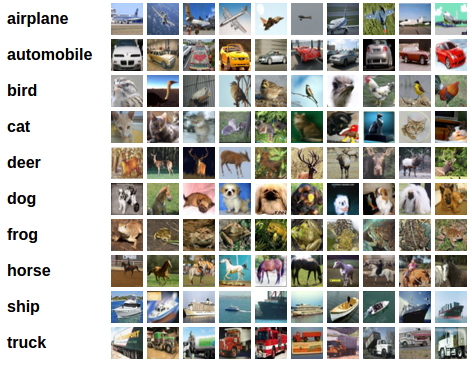
For this tutorial, we will use the CIFAR10 dataset. It has the classes: ‘airplane’, ‘automobile’, ‘bird’, ‘cat’, ‘deer’, ‘dog’, ‘frog’, ‘horse’, ‘ship’, ‘truck’. The images in CIFAR-10 are of size 3x32x32, i.e. 3-channel color images of 32x32 pixels in size.

Training an image classifier

We will do the following steps in order:

Load and normalize the CIFAR10 training and test datasets using torchvision
Define a Convolutional Neural Network
Define a loss function
Train the network on the training data
Test the network on the test data

1. Load and normalize CIFAR10

Using torchvision, it’s extremely easy to load CIFAR10.

import torch
import torchvision
import torchvision.transforms as transforms

The output of torchvision datasets are PILImage images of range [0, 1]. We transform them to Tensors of normalized range [-1, 1].

CodeOut

transform = transforms.Compose(
    [transforms.ToTensor(),
     transforms.Normalize((0.5, 0.5, 0.5), (0.5, 0.5, 0.5))])

batch_size = 4

trainset = torchvision.datasets.CIFAR10(root='./data', train=True,
                                        download=True, transform=transform)
trainloader = torch.utils.data.DataLoader(trainset, batch_size=batch_size,
                                          shuffle=True, num_workers=2)

testset = torchvision.datasets.CIFAR10(root='./data', train=False,
                                       download=True, transform=transform)
testloader = torch.utils.data.DataLoader(testset, batch_size=batch_size,
                                         shuffle=False, num_workers=2)

classes = ('plane', 'car', 'bird', 'cat',
           'deer', 'dog', 'frog', 'horse', 'ship', 'truck')

Downloading https://www.cs.toronto.edu/~kriz/cifar-10-python.tar.gz to ./data/cifar-10-python.tar.gz

  0%|          | 0/170498071 [00:00<?, ?it/s]
  0%|          | 458752/170498071 [00:00<00:41, 4121381.69it/s]
  4%|4         | 6881280/170498071 [00:00<00:04, 37897415.11it/s]
 10%|#         | 17760256/170498071 [00:00<00:02, 69384175.71it/s]
 17%|#6        | 28377088/170498071 [00:00<00:01, 83618503.64it/s]
 23%|##2       | 38699008/170498071 [00:00<00:01, 90536307.86it/s]
 28%|##8       | 48562176/170498071 [00:00<00:01, 93229335.17it/s]
 34%|###4      | 58720256/170498071 [00:00<00:01, 95943506.49it/s]
 41%|####      | 69763072/170498071 [00:00<00:01, 100535136.99it/s]
 48%|####7     | 81100800/170498071 [00:00<00:00, 104503489.28it/s]
 54%|#####4    | 92372992/170498071 [00:01<00:00, 106950067.43it/s]
 61%|######    | 103415808/170498071 [00:01<00:00, 107941908.03it/s]
 67%|######7   | 114458624/170498071 [00:01<00:00, 108650739.76it/s]
 74%|#######3  | 125534208/170498071 [00:01<00:00, 109211172.00it/s]
 80%|########  | 136478720/170498071 [00:01<00:00, 108701673.82it/s]
 86%|########6 | 147357696/170498071 [00:01<00:00, 108282743.98it/s]
 93%|#########2| 158433280/170498071 [00:01<00:00, 109018030.63it/s]
 99%|#########9| 169508864/170498071 [00:01<00:00, 109536448.04it/s]
100%|##########| 170498071/170498071 [00:01<00:00, 98744600.68it/s]
Extracting ./data/cifar-10-python.tar.gz to ./data
Files already downloaded and verified

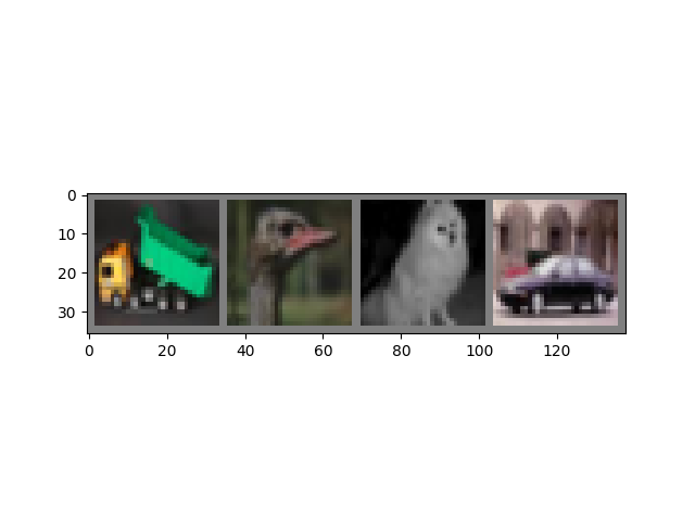
Let us show some of the training images, for fun.

CodeOut

import matplotlib.pyplot as plt
import numpy as np

# functions to show an image


def imshow(img):
    img = img / 2 + 0.5     # unnormalize
    npimg = img.numpy()
    plt.imshow(np.transpose(npimg, (1, 2, 0)))
    plt.show()


# get some random training images
dataiter = iter(trainloader)
images, labels = next(dataiter)

# show images
imshow(torchvision.utils.make_grid(images))
# print labels
print(' '.join(f'{classes[labels[j]]:5s}' for j in range(batch_size)))

truck bird  dog   car

2. Define a Convolutional Neural Network

Copy the neural network from the Neural Networks section before and modify it to take 3-channel images (instead of 1-channel images as it was defined).

import torch.nn as nn
import torch.nn.functional as F


class Net(nn.Module):
    def __init__(self):
        super().__init__()
        self.conv1 = nn.Conv2d(3, 6, 5)
        self.pool = nn.MaxPool2d(2, 2)
        self.conv2 = nn.Conv2d(6, 16, 5)
        self.fc1 = nn.Linear(16 * 5 * 5, 120)
        self.fc2 = nn.Linear(120, 84)
        self.fc3 = nn.Linear(84, 10)

    def forward(self, x):
        x = self.pool(F.relu(self.conv1(x)))
        x = self.pool(F.relu(self.conv2(x)))
        x = torch.flatten(x, 1) # flatten all dimensions except batch
        x = F.relu(self.fc1(x))
        x = F.relu(self.fc2(x))
        x = self.fc3(x)
        return x


net = Net()

3. Define a Loss function and optimizer

Let’s use a Classification Cross-Entropy loss and SGD with momentum.

import torch.optim as optim

criterion = nn.CrossEntropyLoss()
optimizer = optim.SGD(net.parameters(), lr=0.001, momentum=0.9)

4. Train the network

This is when things start to get interesting. We simply have to loop over our data iterator, and feed the inputs to the network and optimize.

CodeOut

for epoch in range(2):  # loop over the dataset multiple times

    running_loss = 0.0
    for i, data in enumerate(trainloader, 0):
        # get the inputs; data is a list of [inputs, labels]
        inputs, labels = data

        # zero the parameter gradients
        optimizer.zero_grad()

        # forward + backward + optimize
        outputs = net(inputs)
        loss = criterion(outputs, labels)
        loss.backward()
        optimizer.step()

        # print statistics
        running_loss += loss.item()
        if i % 2000 == 1999:    # print every 2000 mini-batches
            print(f'[{epoch + 1}, {i + 1:5d}] loss: {running_loss / 2000:.3f}')
            running_loss = 0.0

print('Finished Training')

[1,  2000] loss: 2.219
[1,  4000] loss: 1.909
[1,  6000] loss: 1.690
[1,  8000] loss: 1.565
[1, 10000] loss: 1.533
[1, 12000] loss: 1.482
[2,  2000] loss: 1.423
[2,  4000] loss: 1.385
[2,  6000] loss: 1.368
[2,  8000] loss: 1.327
[2, 10000] loss: 1.324
[2, 12000] loss: 1.316
Finished Training

Let’s quickly save our trained model:

PATH = './cifar_net.pth'
torch.save(net.state_dict(), PATH)

5. Test the network on the test data

We have trained the network for 2 passes over the training dataset. But we need to check if the network has learnt anything at all.

We will check this by predicting the class label that the neural network outputs, and checking it against the ground-truth. If the prediction is correct, we add the sample to the list of correct predictions.

Okay, first step. Let us display an image from the test set to get familiar.

CodeOut

dataiter = iter(testloader)
images, labels = next(dataiter)

# print images
imshow(torchvision.utils.make_grid(images))
print('GroundTruth: ', ' '.join(f'{classes[labels[j]]:5s}' for j in range(4)))

GroundTruth:  cat   ship  ship  plane

Next, let’s load back in our saved model (note: saving and re-loading the model wasn’t necessary here, we only did it to illustrate how to do so):

CodeOut

net = Net()
net.load_state_dict(torch.load(PATH))

<All keys matched successfully>

Okay, now let us see what the neural network thinks these examples above are:

outputs = net(images)

The outputs are energies for the 10 classes. The higher the energy for a class, the more the network thinks that the image is of the particular class. So, let’s get the index of the highest energy:

CodeOut

_, predicted = torch.max(outputs, 1)

print('Predicted: ', ' '.join(f'{classes[predicted[j]]:5s}'
                              for j in range(4)))

Predicted:  cat   plane plane ship

The results seem pretty good.

Let us look at how the network performs on the whole dataset.

CodeOut

correct = 0
total = 0
# since we're not training, we don't need to calculate the gradients for our outputs
with torch.no_grad():
    for data in testloader:
        images, labels = data
        # calculate outputs by running images through the network
        outputs = net(images)
        # the class with the highest energy is what we choose as prediction
        _, predicted = torch.max(outputs.data, 1)
        total += labels.size(0)
        correct += (predicted == labels).sum().item()

print(f'Accuracy of the network on the 10000 test images: {100 * correct // total} %')

Accuracy of the network on the 10000 test images: 54 %

That looks way better than chance, which is 10% accuracy (randomly picking a class out of 10 classes). Seems like the network learnt something.

Hmmm, what are the classes that performed well, and the classes that did not perform well:

CodeOut

# prepare to count predictions for each class
correct_pred = {classname: 0 for classname in classes}
total_pred = {classname: 0 for classname in classes}

# again no gradients needed
with torch.no_grad():
    for data in testloader:
        images, labels = data
        outputs = net(images)
        _, predictions = torch.max(outputs, 1)
        # collect the correct predictions for each class
        for label, prediction in zip(labels, predictions):
            if label == prediction:
                correct_pred[classes[label]] += 1
            total_pred[classes[label]] += 1


# print accuracy for each class
for classname, correct_count in correct_pred.items():
    accuracy = 100 * float(correct_count) / total_pred[classname]
    print(f'Accuracy for class: {classname:5s} is {accuracy:.1f} %')

Accuracy for class: plane is 71.4 %
Accuracy for class: car   is 64.1 %
Accuracy for class: bird  is 37.0 %
Accuracy for class: cat   is 13.3 %
Accuracy for class: deer  is 50.1 %
Accuracy for class: dog   is 54.7 %
Accuracy for class: frog  is 72.4 %
Accuracy for class: horse is 69.3 %
Accuracy for class: ship  is 64.6 %
Accuracy for class: truck is 48.3 %

Okay, so what next?

How do we run these neural networks on the GPU?

Training on GPU

Just like how you transfer a Tensor onto the GPU, you transfer the neural net onto the GPU.

Let’s first define our device as the first visible cuda device if we have CUDA available:

CodeOut

device = torch.device('cuda:0' if torch.cuda.is_available() else 'cpu')

# Assuming that we are on a CUDA machine, this should print a CUDA device:

print(device)

cuda:0

The rest of this section assumes that device is a CUDA device.

Then these methods will recursively go over all modules and convert their parameters and buffers to CUDA tensors:

net.to(device)

Remember that you will have to send the inputs and targets at every step to the GPU too:

inputs, labels = data[0].to(device), data[1].to(device)

Why don’t I notice MASSIVE speedup compared to CPU? Because your network is really small.

Goals achieved:

Understanding PyTorch’s Tensor library and neural networks at a high level.
Train a small neural network to classify images

1. Deep Learning with PyTorch

A Gentle Introduction to torch.autograd

Background

Usage in PyTorch

Differentiation in Autograd

Optional Reading - Vector Calculus using autograd

Computational Graph

Exclusion from the DAG

Neural Networks

Define the network

Loss Function

Backprop

Update the weights

Training a Classifier

What about data?

Training an image classifier

1. Load and normalize CIFAR10

2. Define a Convolutional Neural Network

3. Define a Loss function and optimizer

4. Train the network

5. Test the network on the test data

Training on GPU

References

A Gentle Introduction to `torch.autograd`

Optional Reading - Vector Calculus using `autograd`