3. Datasets & DataLoaders

---

데이터 샘플을 처리하기 위한 코드는 지저분해지고 유지 관리하기 어려울 수 있습니다. 우리는 더 나은 가독성과 모듈성을 위해 데이터 세트 코드를 모델 학습 코드에서 분리하는 것이 이상적입니다. PyTorch는 두 가지 데이터 프리미티브(torch.utils.data.DataLoader 및 torch.utils.data.Dataset)를 제공하므로 사전 로드된 데이터 세트와 자체 데이터를 사용할 수 있습니다. Dataset은 샘플과 해당 레이블을 저장하고 DataLoader는 샘플에 쉽게 액세스할 수 있도록 Dataset 주위에 이터러블을 래핑합니다.

Code for processing data samples can get messy and hard to maintain; we ideally want our dataset code to be decoupled from our model training code for better readability and modularity. PyTorch provides two data primitives: torch.utils.data.DataLoader and torch.utils.data.Dataset that allow you to use pre-loaded datasets as well as your own data. Dataset stores the samples and their corresponding labels, and DataLoader wraps an iterable around the Dataset to enable easy access to the samples.

PyTorch 도메인 라이브러리는 torch.utils.data.Dataset을 하위 클래스로 분류하고 특정 데이터에 특정한 함수를 구현하는 미리 로드된 여러 데이터 세트(예: FashionMNIST)를 제공합니다. 모델을 프로토타입하고 벤치마킹하는 데 사용할 수 있습니다.

PyTorch domain libraries provide a number of pre-loaded datasets (such as FashionMNIST) that subclass torch.utils.data.Dataset and implement functions specific to the particular data. They can be used to prototype and benchmark your model.

Loading a Dataset

다음은 TorchVision에서 Fashion-MNIST 데이터 세트를 로드하는 방법의 예입니다. Fashion-MNIST는 60,000개의 학습 예제와 10,000개의 테스트 예제로 구성된 Zalando의 기사 이미지 데이터 세트입니다. 각 예는 28×28 그레이스케일 이미지와 10개 클래스 중 하나의 관련 레이블로 구성됩니다.

Here is an example of how to load the Fashion-MNIST dataset from TorchVision. Fashion-MNIST is a dataset of Zalando’s article images consisting of 60,000 training examples and 10,000 test examples. Each example comprises a 28×28 grayscale image and an associated label from one of 10 classes.

다음 매개변수를 사용하여 FashionMNIST 데이터세트를 로드합니다:

• root는 학습/테스트 데이터가 저장되는 경로이고,

• train은 학습 또는 테스트 데이터 세트를 지정하고,

• download=True는 root에서 사용할 수 없는 경우 인터넷에서 데이터를 다운로드합니다.

• transform 및 target_transform은 피처 및 레이블 변환을 지정합니다.

We load the FashionMNIST Dataset with the following parameters:

• root is the path where the train/test data is stored,

• train specifies training or test dataset,

• download=True downloads the data from the internet if it’s not available at root.

• transform and target_transform specify the feature and label transformations

CodeOut

import torch
from torch.utils.data import Dataset
from torchvision import datasets
from torchvision.transforms import ToTensor
import matplotlib.pyplot as plt


training_data = datasets.FashionMNIST(
    root="data",
    train=True,
    download=True,
    transform=ToTensor()
)

test_data = datasets.FashionMNIST(
    root="data",
    train=False,
    download=True,
    transform=ToTensor()
)

Downloading http://fashion-mnist.s3-website.eu-central-1.amazonaws.com/train-images-idx3-ubyte.gz
Downloading http://fashion-mnist.s3-website.eu-central-1.amazonaws.com/train-images-idx3-ubyte.gz to data/FashionMNIST/raw/train-images-idx3-ubyte.gz

  0%|          | 0/26421880 [00:00<?, ?it/s]
  0%|          | 32768/26421880 [00:00<01:27, 300571.35it/s]
  0%|          | 65536/26421880 [00:00<01:28, 298648.46it/s]
  0%|          | 131072/26421880 [00:00<01:00, 434666.18it/s]
  1%|          | 229376/26421880 [00:00<00:42, 616267.06it/s]
  2%|1         | 491520/26421880 [00:00<00:20, 1254399.25it/s]
  4%|3         | 950272/26421880 [00:00<00:11, 2248350.72it/s]
  7%|7         | 1933312/26421880 [00:00<00:05, 4436811.04it/s]
 15%|#4        | 3833856/26421880 [00:00<00:02, 8532483.29it/s]
 26%|##6       | 6946816/26421880 [00:00<00:01, 14687982.55it/s]
 38%|###7      | 9928704/26421880 [00:01<00:00, 18536441.65it/s]
 49%|####9     | 13041664/26421880 [00:01<00:00, 21532591.64it/s]
 61%|######1   | 16121856/26421880 [00:01<00:00, 23498842.14it/s]
 72%|#######1  | 19005440/26421880 [00:01<00:00, 24079501.66it/s]
 84%|########3 | 22118400/26421880 [00:01<00:00, 25363999.76it/s]
 95%|#########5| 25231360/26421880 [00:01<00:00, 26227526.23it/s]
100%|##########| 26421880/26421880 [00:01<00:00, 15864756.02it/s]
Extracting data/FashionMNIST/raw/train-images-idx3-ubyte.gz to data/FashionMNIST/raw

Downloading http://fashion-mnist.s3-website.eu-central-1.amazonaws.com/train-labels-idx1-ubyte.gz
Downloading http://fashion-mnist.s3-website.eu-central-1.amazonaws.com/train-labels-idx1-ubyte.gz to data/FashionMNIST/raw/train-labels-idx1-ubyte.gz

  0%|          | 0/29515 [00:00<?, ?it/s]
100%|##########| 29515/29515 [00:00<00:00, 272799.13it/s]
100%|##########| 29515/29515 [00:00<00:00, 271255.74it/s]
Extracting data/FashionMNIST/raw/train-labels-idx1-ubyte.gz to data/FashionMNIST/raw

Downloading http://fashion-mnist.s3-website.eu-central-1.amazonaws.com/t10k-images-idx3-ubyte.gz
Downloading http://fashion-mnist.s3-website.eu-central-1.amazonaws.com/t10k-images-idx3-ubyte.gz to data/FashionMNIST/raw/t10k-images-idx3-ubyte.gz

  0%|          | 0/4422102 [00:00<?, ?it/s]
  1%|          | 32768/4422102 [00:00<00:14, 297104.92it/s]
  1%|1         | 65536/4422102 [00:00<00:14, 295670.57it/s]
  3%|2         | 131072/4422102 [00:00<00:09, 430087.70it/s]
  5%|5         | 229376/4422102 [00:00<00:06, 608622.69it/s]
 10%|9         | 425984/4422102 [00:00<00:03, 1028985.16it/s]
 20%|##        | 884736/4422102 [00:00<00:01, 2079825.49it/s]
 40%|####      | 1769472/4422102 [00:00<00:00, 4008029.25it/s]
 80%|########  | 3538944/4422102 [00:00<00:00, 7798200.16it/s]
100%|##########| 4422102/4422102 [00:00<00:00, 4938713.58it/s]
Extracting data/FashionMNIST/raw/t10k-images-idx3-ubyte.gz to data/FashionMNIST/raw

Downloading http://fashion-mnist.s3-website.eu-central-1.amazonaws.com/t10k-labels-idx1-ubyte.gz
Downloading http://fashion-mnist.s3-website.eu-central-1.amazonaws.com/t10k-labels-idx1-ubyte.gz to data/FashionMNIST/raw/t10k-labels-idx1-ubyte.gz

  0%|          | 0/5148 [00:00<?, ?it/s]
100%|##########| 5148/5148 [00:00<00:00, 22055441.26it/s]
Extracting data/FashionMNIST/raw/t10k-labels-idx1-ubyte.gz to data/FashionMNIST/raw

Iterating and Visualizing the Dataset

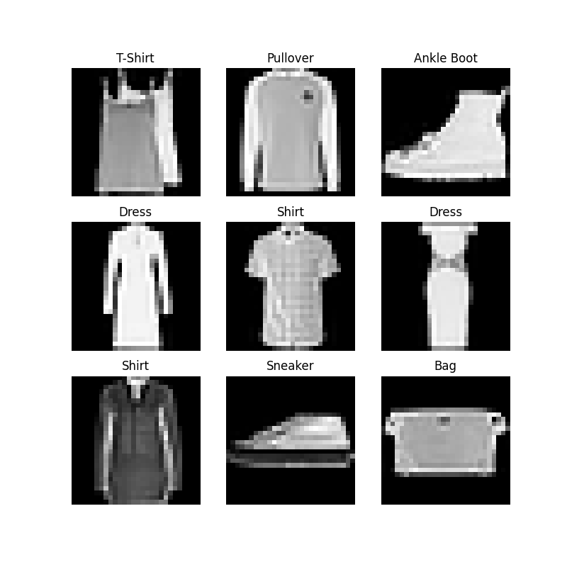
training_data[index] 리스트처럼 수동으로 Datasets를 인덱싱할 수 있습니다. 우리는 학습 데이터의 일부 샘플을 시각화하기 위해 matplotlib를 사용합니다.

We can index Datasets manually like a list: training_data[index]. We use matplotlib to visualize some samples in our training data.

labels_map = {
    0: "T-Shirt",
    1: "Trouser",
    2: "Pullover",
    3: "Dress",
    4: "Coat",
    5: "Sandal",
    6: "Shirt",
    7: "Sneaker",
    8: "Bag",
    9: "Ankle Boot",
}
figure = plt.figure(figsize=(8, 8))
cols, rows = 3, 3
for i in range(1, cols * rows + 1):
    sample_idx = torch.randint(len(training_data), size=(1,)).item()
    img, label = training_data[sample_idx]
    figure.add_subplot(rows, cols, i)
    plt.title(labels_map[label])
    plt.axis("off")
    plt.imshow(img.squeeze(), cmap="gray")
plt.show()

---

Creating a Custom Dataset for your files

사용자 정의 Dataset 클래스는 __init__, __len__ 및 __getitem__의 세 가지 함수를 구현해야 합니다. 이 구현을 살펴보세요; FashionMNIST 이미지는 img_dir 디렉토리에 저장되고 레이블은 CSV 파일 annotations_file에 별도로 저장됩니다.

A custom Dataset class must implement three functions: __init__, __len__, and __getitem__. Take a look at this implementation; the FashionMNIST images are stored in a directory img_dir, and their labels are stored separately in a CSV file annotations_file.

다음 섹션에서는 이러한 각 함수에서 무슨 일이 일어나는지 분석할 것입니다.

In the next sections, we’ll break down what’s happening in each of these functions.

import os
import pandas as pd
from torchvision.io import read_image

class CustomImageDataset(Dataset):
    def __init__(self, annotations_file, img_dir, transform=None, target_transform=None):
        self.img_labels = pd.read_csv(annotations_file)
        self.img_dir = img_dir
        self.transform = transform
        self.target_transform = target_transform

    def __len__(self):
        return len(self.img_labels)

    def __getitem__(self, idx):
        img_path = os.path.join(self.img_dir, self.img_labels.iloc[idx, 0])
        image = read_image(img_path)
        label = self.img_labels.iloc[idx, 1]
        if self.transform:
            image = self.transform(image)
        if self.target_transform:
            label = self.target_transform(label)
        return image, label

__init__

__init__ 함수는 Dataset 객체를 인스턴스화할 때 한 번 실행됩니다. 이미지, 주석 파일 및 두 변환을 모두 포함하는 디렉토리를 초기화합니다(다음 섹션에서 더 자세히 다룹니다).

The __init__ function is run once when instantiating the Dataset object. We initialize the directory containing the images, the annotations file, and both transforms (covered in more detail in the next section).

labels.csv 파일은 다음과 같습니다:

The labels.csv file looks like:

tshirt1.jpg, 0
tshirt2.jpg, 0
......
ankleboot999.jpg, 9

def __init__(self, annotations_file, img_dir, transform=None, target_transform=None):
    self.img_labels = pd.read_csv(annotations_file)
    self.img_dir = img_dir
    self.transform = transform
    self.target_transform = target_transform

__len__

__len__ 함수는 데이터 세트의 샘플 수를 반환합니다.

The __len__ function returns the number of samples in our dataset.

예시:

Example:

def __len__(self):
    return len(self.img_labels)

__getitem__

__getitem__ 함수는 주어진 인덱스 idx에 있는 데이터 세트에서 샘플을 로드하고 반환합니다. 인덱스를 기반으로 디스크에서 이미지의 위치를 식별하고, 이를 read_image를 사용하여 텐서로 변환하고, self.img_labels의 csv 데이터에서 해당 레이블을 검색하고, 변환 함수를 호출하고, 텐서 이미지와 해당 레이블을 튜플로 반환합니다.

The __getitem__ function loads and returns a sample from the dataset at the given index idx. Based on the index, it identifies the image’s location on disk, converts that to a tensor using read_image, retrieves the corresponding label from the csv data in self.img_labels, calls the transform functions on them (if applicable), and returns the tensor image and corresponding label in a tuple.

def __getitem__(self, idx):
    img_path = os.path.join(self.img_dir, self.img_labels.iloc[idx, 0])
    image = read_image(img_path)
    label = self.img_labels.iloc[idx, 1]
    if self.transform:
        image = self.transform(image)
    if self.target_transform:
        label = self.target_transform(label)
    return image, label

---

Preparing your data for training with DataLoaders

Dataset은 데이터 세트의 피처를 검색하고 한 번에 하나의 샘플에 레이블을 지정합니다. 모델을 학습하는 동안 우리는 일반적으로 "미니배치"로 샘플을 전달하고, 모델 과적합을 줄이기 위해 모든 에포크에서 데이터를 다시 섞고, Python의 multiprocessing를 사용하여 데이터 검색 속도를 높이고자 합니다.

The Dataset retrieves our dataset’s features and labels one sample at a time. While training a model, we typically want to pass samples in “minibatches”, reshuffle the data at every epoch to reduce model overfitting, and use Python’s multiprocessing to speed up data retrieval.

DataLoader는 쉬운 API에서 이러한 복잡성을 추상화하는 이터러블입니다.

DataLoader is an iterable that abstracts this complexity for us in an easy API.

from torch.utils.data import DataLoader

train_dataloader = DataLoader(training_data, batch_size=64, shuffle=True)
test_dataloader = DataLoader(test_data, batch_size=64, shuffle=True)

Iterate through the DataLoader

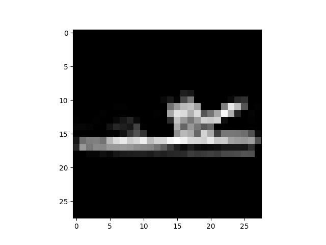
해당 데이터 세트를 DataLoader에 로드했으며 필요에 따라 데이터 세트를 반복할 수 있습니다. 아래의 각 반복은 train_features 및 train_labels의 배치를 반환합니다(각각 batch_size=64 피처 및 레이블 포함). shuffle=True를 지정했기 때문에 모든 배치를 반복한 후 데이터가 섞입니다.

We have loaded that dataset into the DataLoader and can iterate through the dataset as needed. Each iteration below returns a batch of train_features and train_labels (containing batch_size=64 features and labels respectively). Because we specified shuffle=True, after we iterate over all batches the data is shuffled.

CodeOut

# Display image and label.
train_features, train_labels = next(iter(train_dataloader))
print(f"Feature batch shape: {train_features.size()}")
print(f"Labels batch shape: {train_labels.size()}")
img = train_features[0].squeeze()
label = train_labels[0]
plt.imshow(img, cmap="gray")
plt.show()
print(f"Label: {label}")

Feature batch shape: torch.Size([64, 1, 28, 28])
Labels batch shape: torch.Size([64])
Label: 5

---

References

• https://pytorch.org/tutorials/beginner/basics/data_tutorial.html