2. Eigendecomposition
1. 키워드
- Diagonalizable Matrix(대각화행렬)
- Eigendecomposition(고유값 분해): Eigenvector로부터 유도되는 Eigenvalue 행렬과 Eigenvector에 의해 분해될 수 있는 행렬의 표현
2. Diagonalization
We want to change a given square matrix \(A \in \mathbb{R}^{n \times n}\) into a diagonal matrix via \(D=V^{-1} A V\), where \(V \in \mathbb{R}^{n \times n}\) is an ivertible matrix and \(D \in \mathbb{R}^{n \times n}\) is a diagonal matrix. This is called a diagonalization of \(A\).
It is not always possible to diagonalize \(A\). For \(A\) to be diagonalizable, an invertible \(V\) should exist such that \(V^{-1} A V\) becomes a diagonal matrix.
3. Finding \(V\) and \(D\)
How can we find an invertible \(P\) and the resulting diagonal matrix \(D=V^{-1} A V\)?
\(D=V^{-1} A V \Longrightarrow V D=A V\)
Let us represent the following:
Equating columns, we obtain \(A \mathbf{v}_{1}=\lambda_{1} \mathbf{v}_{1}, A \mathbf{v}_{2}=\lambda_{2} \mathbf{v}_{2}, \ldots, A \mathbf{v}_{n}=\lambda_{n} \mathbf{v}_{n}\).
Thus, \(\mathbf{v}_{1}, \mathbf{v}_{2}, \ldots, \mathbf{v}_{n}\) should be eigenvectors and \(\lambda_{1}, \lambda_{2}, \ldots, \lambda_{n}\) should be eigenvalues.
Then, For \(V D=A V \Longrightarrow D=V^{-1} A V\) to be true, \(V\) should invertible.
In this case, the resulting diagonal matrix \(D\) has eigenvalues as diagonal entries.
4. Diagonalizable Matrix
For \(V\) to be invertible, \(V\) should be a square matrix in \(\mathbb{R}^{{n \times n}}\), and \(V\) should have \(n\) linearly indepedent columns.
Recall columns of \(V\) are eigenvectors.
Hence, \(A\) should have \(n\) linearly independent eigenvectors.
It is not always the case, but if it is, \(A\) is diagonalizable.
5. Eigendecomposition
If \(A\) is diagonalizable, we can write \(D=V^{-1} A V\).
We can also write \(A=V D V^{-1}\), which we call eigendecomposition of \(A\).
\(A\) being diagonalizable is equivalent to \(A\) having eigendecomposition.
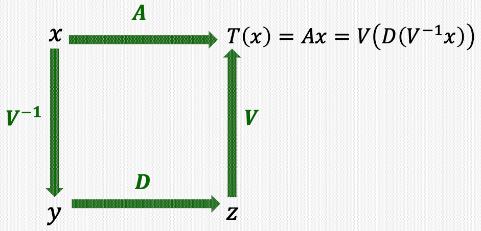
6. Linear Transformation via Eigendecomposition
Suppose \(A\) is diagonalizable, thus having eigendecomposition \(A=V D V^{-1}\).
Consider the linear transformation \(T(\mathbf{x})=A \mathbf{x}\).
\(T(\mathbf{x})=A \mathbf{x}=V D V^{-1} \mathbf{x}=V\left(D\left(V^{-1} \mathbf{x}\right)\right)\)
7. Change of Basis
Suppose \(A \mathbf{v}_{1}=-1 \mathbf{v}_{1}\) and \(A \mathbf{v}_{2}=2 \mathbf{v}_{2}\).
\(T(\mathbf{x})=A \mathbf{x}=V D V^{-1} \mathbf{x}=V\left(D\left({V^{-1} \mathbf{x}}\right)\right)\)
Let \(\mathbf{y}=V^{-1} \mathbf{x}\), then, \(V \mathbf{y}=\mathbf{x}\)
\(\mathbf{y}\) is a new coordinate of \(\mathbf{x}\) with respect to a new basis of eigenvectors \(\left\{\mathbf{v}_{1}, \mathbf{v}_{2}\right\}\).

\(\mathbf{x}=\left[\begin{array}{l}4 \\3\end{array}\right]=4\left[\begin{array}{l}1 \\0\end{array}\right]+3\left[\begin{array}{l}0 \\1\end{array}\right]=\left[\begin{array}{ll}1 & 0 \\0 & 1\end{array}\right]\left[\begin{array}{l}4 \\3\end{array}\right]=P \mathbf{y}=\left[\begin{array}{ll}\mathbf{v}_{1} & \mathbf{v}_{2}\end{array}\right]\left[\begin{array}{l}y_{1} \\y_{2}\end{array}\right]=2 \mathbf{v}_{1}+1 \mathbf{v}_{2} \Rightarrow {\mathbf{y}=\left[\begin{array}{l}2 \\1\end{array}\right]}\)
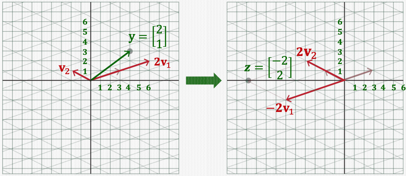
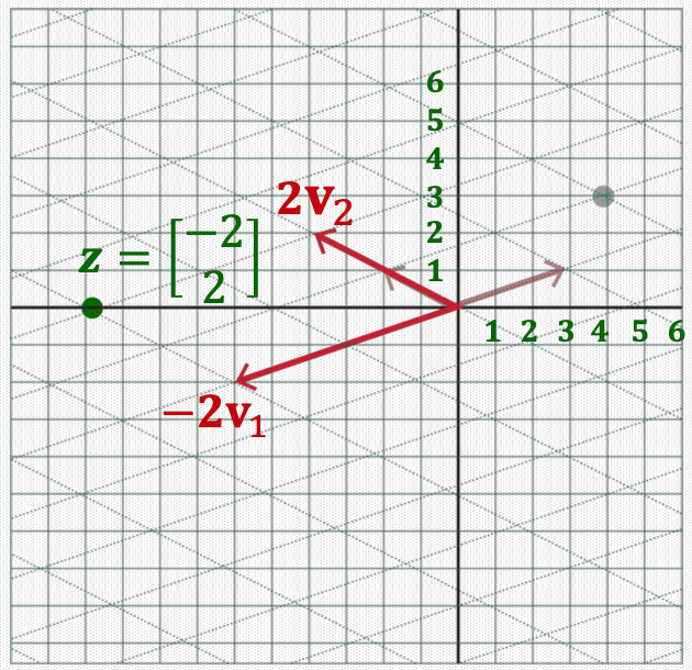
8. Element-wise Scaling
\(T(\mathbf{x})=V\left(D\left({V^{-1} \mathbf{x}}\right)\right)=V({D}{\mathbf{y}})\)\(T(\mathbf{x})=V\left(D\left(V^{-1} \mathbf{x}\right)\right)=V(D \mathbf{y})\)
Let \({z=D} {\mathbf{y}}\), this computation is a simple Element-wise scaling of \({\mathbf{y}}\).
Example: Suppose \({D}=\left[\begin{array}{cc}-1 & 0 \\0 & 2\end{array}\right]\)\(D=\left[\begin{array}{cc}-1 & 0 \\0 & 2\end{array}\right]\).
Then \({z=D} {\mathbf{y}}=\left[\begin{array}{cc}-1 & 0 \\0 & 2\end{array}\right]\left[\begin{array}{l}2 \\1\end{array}\right]=\left[\begin{array}{c}(-1) \times 2 \\2 \times 1\end{array}\right]=\left[\begin{array}{c}-2 \\2\end{array}\right]\)
9. Dimension-wise Scaling
10. Back to Original Basis
\(T(\mathbf{x})=V({D} {\mathbf{y}})=V z\)
\({z}\) is still a coordinate based on the new basis \(\left\{\mathbf{v}_{1}, \mathbf{v}_{2}\right\}\).
\(V {z}\) converts \({z}\) to another coordinates based on the original standard basis.
That is, \(V {z}\)\(V z\) is a linear combination of \(\mathbf{v}_{1}\) and \(\mathbf{v}_{2}\) using the coefficient vector \({z}\).
That is, \(V {z}=\left[\begin{array}{ll}\mathbf{v}_{1} & \mathbf{v}_{2}\end{array}\right]\left[\begin{array}{l}z_{1} \\z_{2}\end{array}\right]=\mathbf{v}_{1} z_{1}+\mathbf{v}_{2} z_{2}\).
\(\begin{aligned}T(\mathbf{x})=& V {z}=\left[\begin{array}{ll}\mathbf{v}_{1} & \mathbf{v}_{2}\end{array}\right]\left[\begin{array}{c}-2 \\2\end{array}\right] =-2 \mathbf{v}_{1}+2 \mathbf{v}_{2} =-2\left[\begin{array}{l}3 \\1\end{array}\right]+2\left[\begin{array}{c}-2 \\1\end{array}\right] =\left[\begin{array}{c}-10 \\0\end{array}\right]\end{aligned}\)
11. Overview of Transformation using Eigendecomposition
12. Linear Transformation via \(A^{k}\)
Now, consider recursive transformation \(A \times A \times \cdots \times A \mathbf{x}=A^{k} \mathbf{x}\).
If \(A\) is diagonalizable, \(A\) has eigendecomposition \(A=V D V^{-1}\).
\(A^{k}=\left(V D V^{-1}\right)\left(V D V^{-1}\right) \cdots\left(V D V^{-1}\right)=V D^{k} V^{-1}\)
\(D^{k}\) is simply computed as \(D^{k}=\left[\begin{array}{cccc}\lambda_{1}^{k} & 0 & \cdots & 0 \\0 & \lambda_{2}^{k} & \ddots & \vdots \\\vdots & \ddots & \ddots & 0 \\0 & \cdots & 0 & \lambda_{n}^{k}\end{array}\right]\).
\(A^{k} \mathbf{x}=V D^{k} V^{-1} \mathbf{x}\) can be computed in the similar manner to the previous example.
It is much faster to compute \(V\left(D^{k}\left(V^{-1} \mathbf{x}\right)\right)\) than to compute \(A^{k} \mathbf{x}\).