1. Eigenvectors and Eigenvalues
1. 키워드
- Eigenvectors(고유벡터): 어떠한 선형변환이 일어난 후에도 방향이 변하지 않는, 0이 아닌 벡터
- Eigenvalues(고유값): 해당 Eigenvector에 대응하는 배수
- Null Space(영공간): 선형변환 후 0 벡터에 매핑되는 Input 공간
- Orthogonal Complement(직교여공간)
2. Eigenvectors and Eigenvalues
Definition: An eigenvector of a square matrix \(A \in \mathbb{R}^{n \times n}\) is a nonzero vector \(\mathbf{x} \in \mathbb{R}^{n}\) such that \(A \mathbf{x}=\lambda \mathbf{x}\) for some scalar \(\lambda\). In this case, \(\lambda\) is called an eigenvalue of \(A\), and such an \(\mathbf{x}\) is called an eigenvector corresponding to \(\lambda\).
3. Transformation Perspective
Consider a linear transformation \(T(\mathbf{x})=A \mathbf{x}\).
If \(\mathbf{x}\) is an eigenvector, then \(T(\mathbf{x})=A \mathbf{x}=\lambda \mathbf{x}\), which means the output vector has the same direction as \(\mathbf{x}\), but the length is scaled by a factor of \(\lambda\).
Example:
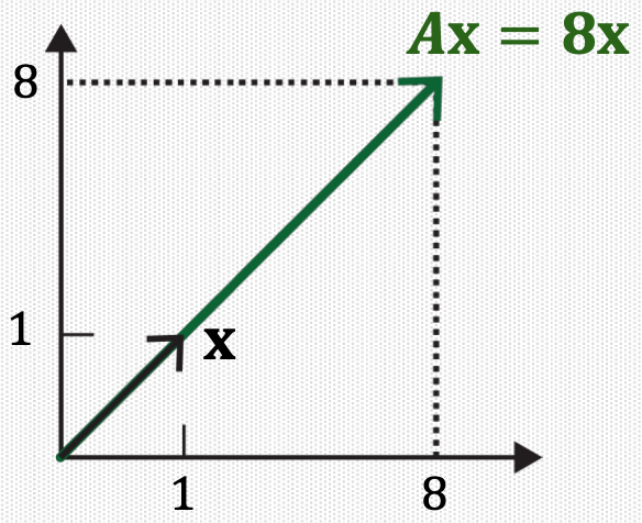
For \(A=\left[\begin{array}{ll}2 & 6 \\ 5 & 3\end{array}\right]\), an eigenvector is \(\left[\begin{array}{l}1 \\ 1\end{array}\right]\) since \(T(\mathbf{x})=A \mathbf{x}=\left[\begin{array}{ll}2 & 6 \\5 & 3\end{array}\right]\left[\begin{array}{l}1 \\1\end{array}\right]=\left[\begin{array}{l}8 \\8\end{array}\right]=8\left[\begin{array}{l}1 \\1\end{array}\right]\)
4. Computational Advantage
Which computation is faster between \(\left[\begin{array}{ll}2 & 6 \\ 5 & 3\end{array}\right]\left[\begin{array}{l}1 \\ 1\end{array}\right]\) and \(8\left[\begin{array}{l}1 \\ 1\end{array}\right]\)?
5. Eigenvectors and Eigenvalues
The equation \(A \mathbf{x}=\lambda \mathbf{x}\) can be re-written as \((A-\lambda I) \mathbf{x}=\mathbf{0}\).
\(\lambda\) is an eigenvalue of an \(n \times n\) matrix \(A\) if and only if this equation has a nontrivial solution (since \(\mathbf{x}\) should be a nonzero vector).
\((A-\lambda I) \mathbf{x}=\mathbf{0}\)
The set of all solutions of the above equation is the null space of the matrix \((A-\lambda I)\), which we call the eigenspace of \(A\) corresponding to \(\lambda\).
The eigenspace consists of the zero vector and all the eigenvectors corresponding to \(\lambda\), satisfying the above equation.
6. Null Space
Definition: The null space of a matrix \(A \in \mathbb{R}^{m \times n}\) is the set of all solutions of a homogeneous linear system, \(A \mathbf{x}=\mathbf{0}\).
We denote the null space of \(A\) as \(\operatorname{Nul}A\).
For \(A=\left[\begin{array}{c}\mathbf{a}_{1}^{T} \\\mathbf{a}_{2}^{T} \\\vdots \\\mathbf{a}_{m}^{T}\end{array}\right]\), \(\mathbf{x}\) should satisfy \(\mathbf{a}_{1}^{T} \mathbf{x}=0, \mathbf{a}_{2}^{T} \mathbf{x}=0, \ldots, \mathbf{a}_{m}^{T} \mathbf{x}=0\).
That is, \(\mathbf{x}\) should be orthogonal to every row vector in \(A\).
7. Null Space is a Subspace
Theorem: The null space of a matrix \(A \in \mathbb{R}^{m \times n}\), denoted as \(\operatorname{Nul}A\) is a subspace of \(\mathbb{R}^{n}\). In other words, the set of all the solutions of a system \(A \mathbf{x}=\mathbf{0}\) is a subspace of \(\mathbb{R}^{n}\).
Note: An eigenspace thus have a set of basis vectors with a particular dimension.
8. Orthogonal Complement
If a vector \(\mathbf{z}\) is orthogonal to every vector in a subspace \(W\) of \(\mathbb{R}^{n}\), then \(\mathbf{z}\) is said to be orthogonal to \(W\).
The set of all vectors \(\mathbf{z}\) that are orthogonal to \(W\) is called the orthogonal complement of \(W\) and is denoted by \(W^{\perp}\) (and read as "\(W\) perpendicular" or simple "W perp").
A vector \(\mathbf{x} \in \mathbb{R}^{n}\) is in \(W^{\perp}\) if and only if \(\mathbf{x}\) is orthogonal to every vector in a set that spans \(W\).
\(W^{\perp}\) is a subspace of \(\mathbb{R}^{n}\).
\(\operatorname{Nul}A=(\operatorname{Row}A)^{\perp}\).
Likewise, \(\operatorname{Nul}A^{T}=(\operatorname{Col}A)^{\perp}\).
9. Fundamental Subspaces Given by \(A\)
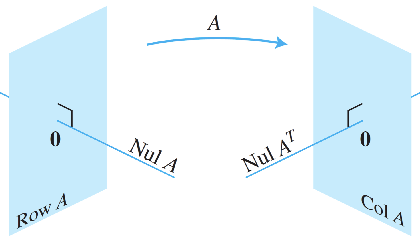
Figure 8 The fundamental subspaces determined by an \(m \times n\) matrix \(A\).
\(\operatorname{Nul}A=(\operatorname{Row}A)^{\perp}\).
\(\operatorname{Nul}A^{T} =(\operatorname{Col}A)^{\perp}\).
10. Example: Eigenvalues and Eigenvectors
Example: Show that \(8\) is an eigenvalue of a matrix \(A=\left[\begin{array}{ll}2 & 6 \\ 5 & 3\end{array}\right]\) and find the corresponding eigenvectors.
Solution: The scalar 8 i an eigenvalue of \(A\) if and only if the equation \((A-8 I) \mathbf{x}=\mathbf{0}\) has a nontrivial solution:
The solution is \(\mathbf{x}=c\left[\begin{array}{l}1 \\ 1\end{array}\right]\) for any nonzero scalar \(c\), which is \(\operatorname{Span}\left\{\left[\begin{array}{l}1 \\ 1\end{array}\right]\right\}\).
In the previous example, \(-3\) is also an eigenvalue:
The solution is \(\mathbf{x}=c\left[\begin{array}{c}1 \\ -5 / 6\end{array}\right]\) for any nonzero scalar \(c\), which is \(\operatorname{Span}\left\{\left[\begin{array}{c}1 \\ -5 / 6\end{array}\right]\right\}\).
11. Characteristic Equation
How can we find the eigenvalues such as \(8\) and \(-3\)?
If \((A-\lambda I) \mathbf{x}=\mathbf{0}\) has a nontrivial solution, then the columns of \((A-\lambda I)\) should be noninvertible.
If it is invertible, \(\mathbf{x}\) cannot be a nonzero vector since \((A-\lambda I)^{-1}(A-\lambda I) \mathbf{x}=(A-\lambda I)^{-1} \mathbf{0} \Longrightarrow \mathbf{x}=\mathbf{0}\).
Thus, we can obtain eigenvalues by solving \(\operatorname{det}(A-\lambda I)=0\) called a characteristic equation.
Also, the solution is not unique, and thus \(A-\lambda I\) has linearly dependent columns.
12. Example: Characteristic Equation
In the previous example, \(A=\left[\begin{array}{ll}2 & 6 \\ 5 & 3\end{array}\right]\) is originally invertible since \(\operatorname{det}(A)=\operatorname{det}\left[\begin{array}{ll}2 & 6 \\5 & 3\end{array}\right]=6-30=-24 \neq 0\).
By solving the characteristic equation, we want to find \(\lambda\) that makes \(A-\lambda I\) non-invertible:
Once obtaining eigenvalues, we compute the eigenvectors for each \(\lambda\) by solving \((A-\lambda I) \mathbf{x}=\mathbf{0}\)
13. Eigenspace
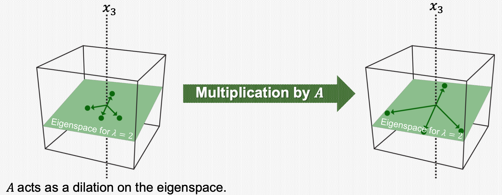
Note that the dimension of the eigenspace (corresponding to a particular \(\lambda\)) can be more than one.
In this case, any vector in the eigenspace satisfies \(T(\mathbf{x})=A \mathbf{x}=\lambda \mathbf{x}\).
14. Finding all eigenvalues and eigenvectors
In summary, we can find all the possible eigenvalues and eigenvectors, as follows.
First, find all the eigenvalue by solving the characteristic equation:
Second, for each eigenvalue \(\lambda\), solve for \((A-\lambda I) \mathbf{x}=\mathbf{0}\) and obtain the set of basis vectors of the corresponding eigenspace.