4. Orthogonalization
1. 키워드
- Gram-Shmidt Orthogonalization(그람-슈미트 직교화)
- QR Factorization(QR분해)
2. Gram-Shmidt Orthogonalization
Example 1: Let \(W=\) \(\operatorname{Span}\left\{\mathbf{x}_{1}, \mathbf{x}_{2}\right\}\), where \(\mathbf{x}_{1}=\left[\begin{array}{l}3 \\6 \\0\end{array}\right]\) and \(\mathbf{x}_{2}=\left[\begin{array}{l}1 \\2 \\2\end{array}\right]\).
Construct an orthogonal basis \(\left\{\mathbf{v}_{1}, \mathbf{v}_{2}\right\}\) for \(W\).
Solution: Let \(\mathbf{v}_{1}=\mathbf{x}_{1}\). Next, Let \(\mathbf{v}_{2}\) the component of \(\mathbf{x}_{2}\) orthogonal to \(\mathbf{x}_{1}\), i.e., \(\mathbf{v}_{2}=\mathbf{x}_{2}-\frac{\mathbf{x}_{2} \cdot \mathbf{x}_{1}}{\mathbf{x}_{1} \cdot \mathbf{x}_{1}} \mathbf{x}_{1}=\left[\begin{array}{l}1 \\2 \\2\end{array}\right]-\frac{15}{45}\left[\begin{array}{l}3 \\6 \\0\end{array}\right]=\left[\begin{array}{l}0 \\0 \\2\end{array}\right]\).
The set \(\left\{\mathbf{x}_{1}, \mathbf{x}_{2}\right\}\) is an orthogonal basis for \(W\).
Example 2: Let \(\mathbf{x}_{1}=\left[\begin{array}{l}1 \\1 \\1 \\1\end{array}\right]\), \(\mathbf{x}_{2}=\left[\begin{array}{l}0 \\1 \\1 \\1\end{array}\right]\), and \(\mathbf{x}_{3}=\left[\begin{array}{l}0 \\0 \\1 \\1\end{array}\right]\). Then \(\left\{\mathbf{x}_{1}, \mathbf{x}_{2},\mathbf{x}_{3}\right\}\) is clearly linearly independent and thus is a basis for a subspace \(W\) of \(\mathbb{R}^{4}\). Construct an orthogonal basis for \(W\).
Solution:
Step 1: Let \(\mathbf{v}_{1}=\mathbf{x}_{1}\) and \(W_{1}=\operatorname{Span}\left\{\mathbf{x}_{1}\right\}=\operatorname{Span}\left\{\mathbf{v}_{1}\right\}\).
Step 2: Let \(\mathbf{v}_{2}\) be the vector produced by subtracting from \(\mathbf{x}_{2}\) its projection onto the subspace \(W_{1}\). That is, let \(\mathbf{v}_{2}=\mathbf{x}_{2}-\operatorname{proj}_{W_{1}} \mathbf{x}_{2}=\mathbf{x}_{2}-\frac{\mathbf{x}_{2} \cdot \mathbf{v}_{1}}{\mathbf{v}_{1} \cdot \mathbf{v}_{1}} \mathbf{v}_{1}=\left[\begin{array}{c}-3 / 4 \\1 / 4 \\1 / 4 \\1 / 4\end{array}\right]\)
\(\mathbf{v}_{2}\) is the component of \(\mathbf{x}_{2}\) orthogonal to \(\mathbf{x}_{1}\), and \(\left\{\mathbf{v}_{1}, \mathbf{v}_{2}\right\}\) is an orthogonal basis for the subspace \(W_{2}\) spanned by \(\mathbf{x}_{1}\) and \(\mathbf{x}_{2}\).
Step 2' (optional): If appropriate, scale \(\mathbf{v}_{2}\) to simplify later computations, e.g., \(\mathbf{v}_{2}=\left[\begin{array}{c}-3 / 4 \\1 / 4 \\1 / 4 \\1 / 4\end{array}\right] \rightarrow \mathbf{v}_{2}^{\prime}=\left[\begin{array}{c}-3 \\1 \\1 \\1\end{array}\right]\)
Step 3: Let \(\mathbf{v}_{3}\) be the vector produced by subtracting from \(\mathbf{x}_{3}\) its projection onto the subspace \(W_{2}\). Use the orthogonal basis \(\left\{\mathbf{v}_{1}, \mathbf{v}_{2}^{\prime}\right\}\) to compute this projection onto \(W_{2}\):
Then \(\mathbf{v}_{3}\) is the component \(\mathbf{x}_{3}\) orthogonal to \(W_{2}\), namely \(\mathbf{v}_{3}=\mathbf{x}_{3}-\operatorname{proj}_{W_{2}} \mathbf{x}_{3}=\left[\begin{array}{c}0 \\-2 / 3 \\1 / 3 \\1 / 3\end{array}\right]\).
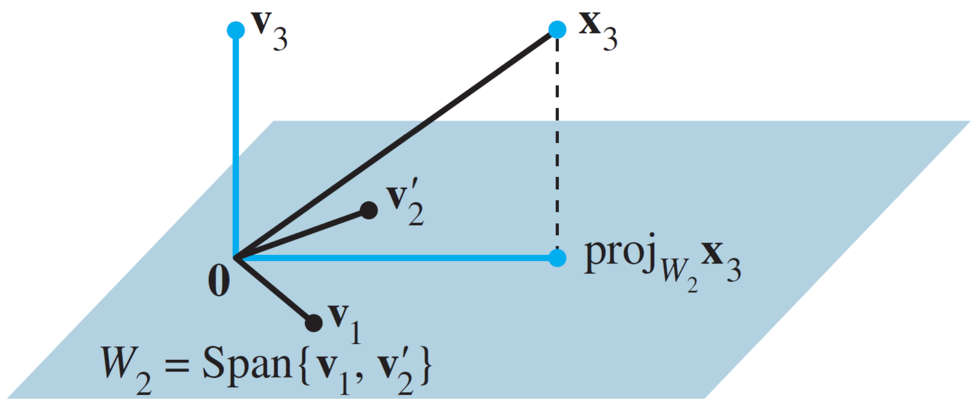
Figure 2 The construction of \(\mathbf{v}_{3}\) from \(\mathbf{x}_{3}\) and \(W_{2}\).
3. QR Factorization
If \(A\) is an \(m \times n\) matrix with linearly independent columns, then \(A\) can be factored as \(A=QR\), where \(Q\) is an \(m \times n\) matrix whose columns form an orthonormal basis for \(\operatorname{Col}A\) and \(R\) is an \(n \times n\) upper triangular invertible matrix with positive entries on its diagonal.
4. Computing QR Factorization
Step 1 (Construction of \(Q\)): The columns of \(A\) form a basis for \(\operatorname{Col}A\) since they are linearly independent. Let these columns be \(\left\{\mathbf{x}_{1}, \ldots, \mathbf{x}_{n}\right\}\). Then, we can construct the orthonormal basis \(\left\{\mathbf{u}_{1}, \ldots, \mathbf{u}_{n}\right\}\) for \(\operatorname{Col}A\) by the Gram-Shmidt process described by Theorem 11. Using this basis, we can construct \(Q\) as \(Q=\left[\begin{array}{llll}\mathbf{u}_{1} & \mathbf{u}_{2} & \cdots & \mathbf{u}_{n}\end{array}\right]\)
Step 2 (Contruction of \(R\)): From (1) in Theorem 11, for \(k=1,\ldots,n,\mathbf{x}_{k}\) is in \(\operatorname{Span}\left\{\mathbf{x}_{1}, \ldots, \mathbf{x}_{k}\right\}=\operatorname{Span}\left\{\mathbf{u}_{1}, \ldots, \mathbf{u}_{k}\right\}\). Therefore, there exist constants \(r_{1 k}, \ldots, r_{k k}\) such that \(\mathbf{x}_{k}=r_{1 k} \mathbf{u}_{1}+\cdots+r_{k k} \mathbf{u}_{k}+0 \cdot \mathbf{u}_{k+1}+\cdots+0 \cdot \mathbf{u}_{n}\)
We can always make \(r_{k k} \geq 0\) because if \(r_{k k}<0\), then we can multiply both \(r_{k k}\) and \(\mathbf{u}_{k}\) by \(-1\). Using this linear combination representation, we can construct \(r_{k}\), the \(k\)-th column of \(R\), as \(\mathbf{r}_{k}=\left[\begin{array}{c}r_{1 k} \\\vdots \\r_{k k} \\0 \\\vdots \\0\end{array}\right]\).
That is, \(\mathbf{x}_{k}=Q \mathbf{r}_{k}\) for \(k=1, \ldots, n\). Let \(R=\left[\begin{array}{lll}\mathbf{r}_{1} & \cdots & \mathbf{r}_{n}\end{array}\right]\). Then, \(A=\left[\begin{array}{lll}\mathbf{x}_{1} & \cdots & \mathbf{x}_{n}\end{array}\right]=\left[\begin{array}{lll}Q \mathbf{r}_{1} & \cdots & Q \mathbf{r}_{n}\end{array}\right]=Q R\).
The fact that \(R\) is invertible follows easily from the fact that the columns of \(A\) are linearly independent (Exercise 19). Since \(R\) is clearly upper triangular (from the previous slide) and invertible, the diagonal entries \(r_{k k}\)'s should be nonzero. By combining this with the fact that \(r_{k k} \geq 0\), \(r_{k k}\)'s must be positive.
5. Example: QR Factorization
Example 4: Find a QR factorization of \(A=\left[\begin{array}{lll}1 & 0 & 0 \\1 & 1 & 0 \\1 & 1 & 1 \\1 & 1 & 1\end{array}\right]\).
Solution: Let \(A=\left[\begin{array}{lll}\mathbf{X}_{1} & \mathbf{X}_{2} & \mathbf{X}_{3}\end{array}\right]\). We first obtain \(\mathbf{v}_{1}=\mathbf{x}_{1}\) and its normalized vector is \(\mathbf{u}_{1}=\left[\begin{array}{l} 1 / 2 \\ 1 / 2 \\ 1 / 2 \\ 1 / 2 \end{array}\right]\).
Thus, \(\mathbf{x}_{1}=2 \mathbf{u}_{1}\), which gives us \(\mathbf{r}_{11}=2\), i.e., \(r_{1}=\left[\begin{array}{l}2 \\0 \\0\end{array}\right]\).
Next, we obtain \(\mathbf{v}_{3}\) as \(\mathbf{v}_{3}=\mathbf{x}_{3}-\operatorname{proj}_{W_{2}} \mathbf{x}_{3}=\mathbf{x}_{3}-\frac{\mathbf{x}_{3} \cdot \mathbf{u}_{1}}{\mathbf{u}_{1} \cdot \mathbf{u}_{1}} \mathbf{u}_{1}-\frac{\mathbf{x}_{3} \cdot \mathbf{u}_{2}}{\mathbf{u}_{2} \cdot \mathbf{u}_{2}} \mathbf{u}_{2}=\left[\begin{array}{l}0 \\0 \\1 \\1\end{array}\right]-1\left[\begin{array}{l}1 / 2 \\1 / 2 \\1 / 2 \\1 / 2\end{array}\right]-\frac{2}{\sqrt{12}}\left[\begin{array}{c}-3 / \sqrt{12} \\1 / \sqrt{12} \\1 / \sqrt{12} \\1 / \sqrt{12}\end{array}\right]=\left[\begin{array}{c}0 \\-2 / 3 \\1 / 3 \\1 / 3\end{array}\right]\) and its normalized vector \(\mathbf{u}_{2}\) as \(\mathbf{u}_{2}=\left[\begin{array}{c}0 \\-2 / \sqrt{6} \\1 / \sqrt{6}\\1 / \sqrt{6}\end{array}\right]\).
Thus, \(\mathbf{x}_{3}=1 \mathbf{u}_{1}+\frac{2}{\sqrt{12}} \mathbf{u}_{2}+\frac{2}{\sqrt{6}} \mathbf{u}_{3}\), i.e., \(\mathbf{r}_{3}=\left[\begin{array}{c}1 \\2 / \sqrt{12} \\2 / \sqrt{6}\end{array}\right]\).
In conclusion, \(Q=\left[\begin{array}{lll}\mathbf{u}_{1} & \mathbf{u}_{2} & \mathbf{u}_{3}\end{array}\right]=\left[\begin{array}{ccc}1 / 2 & -3 / \sqrt{12} & 0 \\1 / 2 & 1 / \sqrt{12} & -2 / \sqrt{6} \\1 / 2 & 1 / \sqrt{12} & 1 / \sqrt{6} \\1 / 2 & 1 / \sqrt{12} & 1 / \sqrt{6}\end{array}\right]\) and \(R=\left[\begin{array}{lll}\mathbf{r}_{1} & \mathbf{r}_{2} & \mathbf{r}_{3}\end{array}\right]=\left[\begin{array}{ccc}2 & -3 / 2 & 1 \\0 & -3 / \sqrt{12} & 2 / \sqrt{12} \\0 & 0 & 2 / \sqrt{6}\end{array}\right]\).