3. Orthogonal Projection
1. 키워드
- Orthogonality
- Orthonormality
- Orthogonal Basis(직교기저)
- Orthonormal Basis(정규직교기저)
- Orthogonal Projection(정사영)
2. Orthogonal Projection Perspective
Back to the case of invertible \(C=A^{T} A\), consider the orthogonal projection of \(\mathbf{b}\) onto \(\operatorname{Col}A\) as \(\hat{\mathbf{b}}=f(\mathbf{b})=A \hat{\mathbf{x}}=A\left(A^{T} A\right)^{-1} A^{T} \mathbf{b}\).
3. Orthogonal and Orthonormal Sets
Definition: A set of vectors \(\left\{\mathbf{u}_{1}, \ldots, \mathbf{u}_{p}\right\}\) in \(\mathbb{R}^{n}\) is an orthogonal set if each pair of distinct vectors from the set is orthogonal, that is, if \(\mathbf{u}_{i} \cdot \mathbf{u}_{j}=0\) whenever \(i \neq j\).
Definition: A set of vectors \(\left\{\mathbf{u}_{1}, \ldots, \mathbf{u}_{p}\right\}\) in \(\mathbb{R}^{n}\) is an orthonormal set if it is an orthogonal set of unit vectors.
Is an orthogonal (or orthonormal) set also a linearly independent set? What about its converse?
4. Orthogonal and Orthonormal Basis
Consider basis \(\left\{\mathbf{u}_{1}, \ldots, \mathbf{u}_{p}\right\}\) of a \(p\)-dimensional subspace \(W\) in \(\mathbb{R}^{n}\).
Can we make it as an orthogonal (or orthonormal) basis?
- Yes, it can be done by Gram-Schmidt process. → QR factorization.
Given the orthogonal basis \(\left\{\mathbf{u}_{1}, \ldots, \mathbf{u}_{p}\right\}\) of \(W\), let's compute the orthogonal projection of \(\mathbf{y} \in \mathbb{R}^{r}\) onto \(W\).
5. Orthogonal Projection \(\hat{\mathbf{y}}\) of \(\mathbf{y}\) onto Line
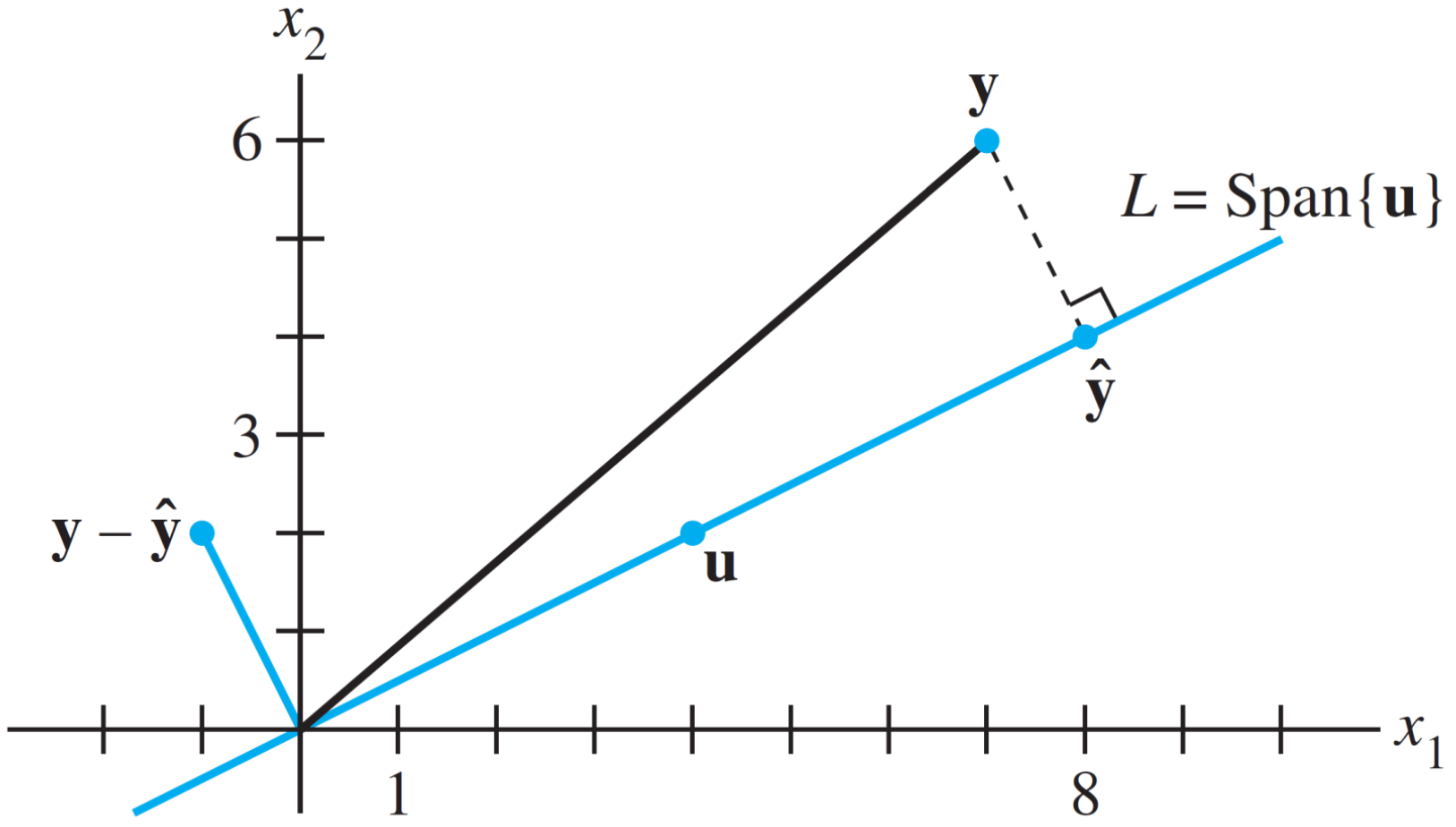
Consider the orthogonal projection \(\hat{\mathbf{y}}\) of \(\mathbf{y}\) onto one-dimensional subspace \(L\).
\(\hat{\mathbf{y}}=\operatorname{proj}_{L} \mathbf{y}=\frac{\mathbf{y} \cdot \mathbf{u}}{\mathbf{u} \cdot \mathbf{u}} \mathbf{u}\)
If \(\mathbf{u}\) is a unit vector, \(\hat{\mathbf{y}}=\operatorname{proj}_{L} \mathbf{y}=(\mathbf{y} \cdot \mathbf{u}) \mathbf{u}\).
6. Orthogonal Projection \(\hat{\mathbf{y}}\) of \(\mathbf{y}\) onto Plane
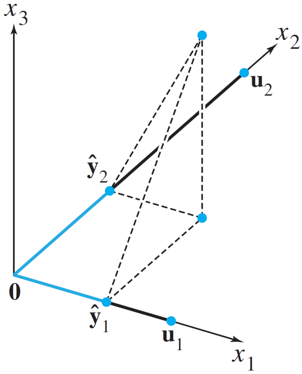
Consider the orthogonal projection \(\hat{\mathbf{y}}\) of \(\mathbf{y}\) onto two-dimensional subspace \(W\).
\(\hat{\mathbf{y}}=\operatorname{proj}_{L} \mathbf{y}=\frac{\mathbf{y} \cdot \mathbf{u}_{1}}{\mathbf{u}_{1} \cdot \mathbf{u}_{1}} \mathbf{u}_{1}+\frac{\mathbf{y} \cdot \mathbf{u}_{2}}{\mathbf{u}_{2} \cdot \mathbf{u}_{2}} \mathbf{u}_{2}\)
If \(\mathbf{u}_{1}\) and \(\mathbf{u}_{2}\) are unit vectors, \(\hat{\mathbf{y}}=\operatorname{proj}_{L} \mathbf{y}=\left(\mathbf{y} \cdot \mathbf{u}_{1}\right) \mathbf{u}_{1}+\left(\mathbf{y} \cdot \mathbf{u}_{2}\right) \mathbf{u}_{2}\).
Projection is done independently on each orthogonal basis vector.
7. Orthogonal Projection when \(\mathbf{y} \in W\)

Consider the orthogonal projection \(\hat{\mathbf{y}}\) of \(\mathbf{y}\) onto two-dimensional subspace \(W\), where \({\mathbf{y} \in W}\).
\(\hat{\mathbf{y}}=\operatorname{proj}_{L} \mathbf{y}{=\mathbf{y}}=\frac{\mathbf{y} \cdot \mathbf{u}_{1}}{\mathbf{u}_{1} \cdot \mathbf{u}_{1}} \mathbf{u}_{1}+\frac{\mathbf{y} \cdot \mathbf{u}_{2}}{\mathbf{u}_{2} \cdot \mathbf{u}_{2}} \mathbf{u}_{2}\)
If \(\mathbf{u}_{1}\) and \(\mathbf{u}_{2}\) are unit vectors, \(\hat{\mathbf{y}}= \mathbf{y}=\left(\mathbf{y} \cdot \mathbf{u}_{1}\right) \mathbf{u}_{1}+\left(\mathbf{y} \cdot \mathbf{u}_{2}\right) \mathbf{u}_{2}\).
The solution is the same as before. Why?
8. Transformation: Orthogonal Projection
Consider a transformation of orthogonal projection \(\hat{\mathbf{b}}\) of \(\mathbf{b}\), given orthonormal basis \(\left\{\mathbf{u}_{1}, \mathbf{u}_{2}\right\}\) of a subspace \(W\):
9. Orthogonal Projection Perspective
Let's verify the following, when \(A=U=\left[\begin{array}{ll}\mathbf{u}_{1} & \mathbf{u}_{2}\end{array}\right]\) has orthonormal columns.
- Back to the case of invertible \(C=A^{T} A\), consider the orthogonal projection of \(\mathbf{b}\) onto \(\operatorname{Col}A\) as \(\hat{\mathbf{b}}=A \hat{\mathbf{x}}=A\left(A^{T} A\right)^{-1} A^{T} \mathbf{b}=f(\mathbf{b})\).
\(C=A^{T} A=\left[\begin{array}{l}\mathbf{u}_{1}^{T} \\\mathbf{u}_{2}^{T}\end{array}\right]\left[\begin{array}{ll}\mathbf{u}_{1} & \mathbf{u}_{2}\end{array}\right]=I\). Thus, \(\hat{\mathbf{b}}=A \hat{\mathbf{x}}=A\left(A^{T} A\right)^{-1} A^{T} \mathbf{b}=A(I)^{-1} A^{T} \mathbf{b}=A A^{T} \mathbf{b}=U U^{T} \mathbf{b}\)