2. Normal Equation
1. 키워드
- Normal Equation(정규방정식): 특정 선형 회귀 문제에서 파라미터의 최적값을 구하는 방법
2. Least Squares Problem
Now, the sum of squared errors can be represented as \(\|\mathbf{b}-A \mathbf{x}\|\).
Definition: Given an overdetermined system \(A \mathbf{x} \simeq \mathbf{b}\) where \(A \in \mathbb{R}^{m \times n}\), \(\mathbf{b} \in \mathbb{R}^{n}\), and \(m \gg n\), a least squares solution \(\hat{\mathbf{X}}\) is defined as \(\hat{\mathbf{x}}=\arg \min _{\mathbf{x}}\|\mathbf{b}-A \mathbf{x}\|\).
The most important aspect of the least squares problem is that no matter what \(\mathbf{x}\) we select, the vector \(A \mathbf{x}\) will necessarily be in the column space \(\operatorname{Col}A\).
Thus, we seek for \(\mathbf{x}\) that makes \(A \mathbf{x}\) as the closest point in \(\operatorname{Col}A\) to \(\mathbf{b}\).
3. Geometric Interpretation of Least Squares
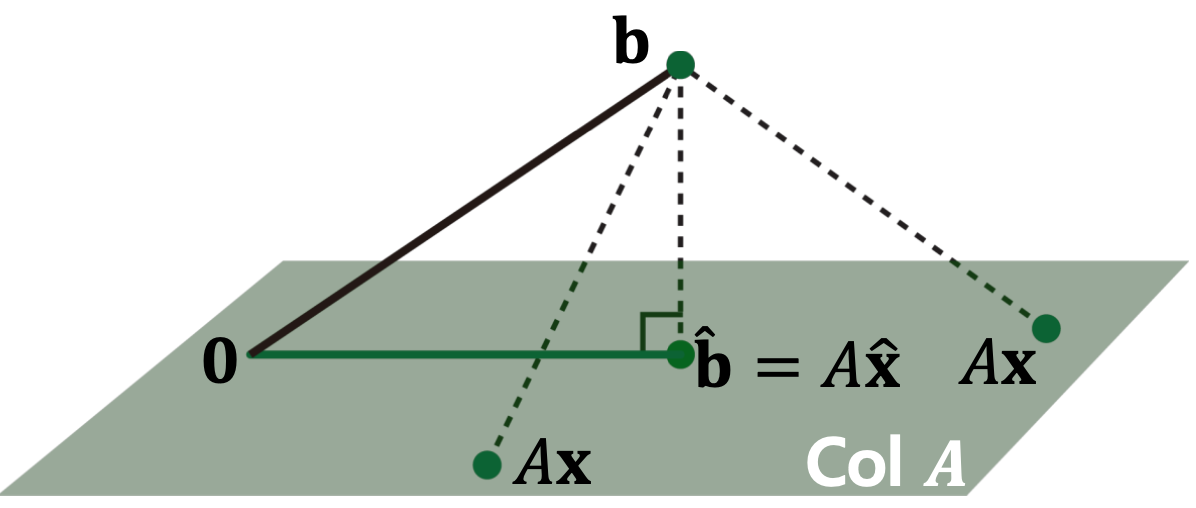
Consider \(\hat{\mathbf{x}}\) such that \(\hat{\mathbf{b}}=A \hat{\mathbf{x}}\) is the closest point to \(\mathbf{b}\) among all points in \(\operatorname{Col}A\).
That is, \(\mathbf{b}\) is closer to \(\hat{\mathbf{b}}\) than to \(A \mathbf{x}\) for any other \(\mathbf{x}\).
To satisfy this, the vector \(\mathbf{b}-A \hat{\mathbf{x}}\) should be orthogonal to \(\operatorname{Col}A\).
This means \(\mathbf{b}-A \hat{\mathbf{x}}\) should be orthogonal to any vector in \(\operatorname{Col}A\):
Or equivalently,
\(\begin{gathered}(\mathbf{b}-A \hat{\mathbf{x}}) \perp \mathbf{a}_{1} \\(\mathbf{b}-A \hat{\mathbf{x}}) \perp \mathbf{a}_{2} \\\vdots \\(\mathbf{b}-A \hat{\mathbf{x}}) \perp \mathbf{a}_{m}\end{gathered}\) → \(\begin{gathered}\mathbf{a}_{1}^{T}(\mathbf{b}-A \widehat{\mathbf{x}})=0 \\\mathbf{a}_{2}^{T}(\mathbf{b}-A \widehat{\mathbf{x}})=0 \\\vdots \\\mathbf{a}_{m}^{T}(\mathbf{b}-A \widehat{\mathbf{x}})=0\end{gathered}\) → \(A^{T}(\mathbf{b}-A \hat{\mathbf{x}})=0\)
4. Normal Equation
Finally, given a least squares problem, \(A \mathbf{x} \simeq \mathbf{b}\), we obtain \(A^{T} A \hat{\mathbf{x}}=A^{T} \mathbf{b}\), which is called a normal equation.
This can be viewed as a new linear system, \(C \mathbf{x}=\mathbf{d}\), where a square matrix \(C=A^{T} A \in \mathbb{R}^{n \times n}\), and \(\mathbf{d}=A^{T} \mathbf{b} \in \mathbb{R}^{n}\).
If \(C=A^{T} A\) is invertible, then the solution is computed as \(\hat{\mathbf{x}}=\left(A^{T} A\right)^{-1} A^{T} \mathbf{b}\).
5. Life-Span Example
\(\left[\begin{array}{lll}60 & 5.5 & 1 \\65 & 5.0 & 0 \\55 & 6.0 & 1 \\50 & 5.0 & 1\end{array}\right]\left[\begin{array}{l}x_{1} \\x_{2} \\x_{3}\end{array}\right]=\left[\begin{array}{l}66 \\74 \\78 \\72\end{array}\right]\)
The normal equation \(A^{T} A \hat{\mathbf{x}}=A^{T} \mathbf{b}\) is \(\left[\begin{array}{cccc}60 & 65 & 55 & 50 \\5.5 & 5.0 & 6.0 & 5.0 \\1 & 0 & 1 & 1\end{array}\right]\left[\begin{array}{ccc}60 & 5.5 & 1 \\65 & 5.0 & 0 \\55 & 6.0 & 1 \\50 & 5.0 & 1\end{array}\right]\left[\begin{array}{l}x_{1} \\x_{2} \\x_{3}\end{array}\right]=\left[\begin{array}{cccc}60 & 65 & 55 & 50 \\5.5 & 5.0 & 6.0 & 5.0 \\1 & 0 & 1 & 1\end{array}\right]\left[\begin{array}{l}66 \\74 \\78 \\72\end{array}\right]\)
\(\left[\begin{array}{ccc}13350 & 1235 & 165 \\1235 & 116.25 & 16.5 \\165 & 16.5 & 3\end{array}\right]\left[\begin{array}{l}x_{1} \\x_{2} \\x_{3}\end{array}\right]=\left[\begin{array}{c}16600 \\1561 \\216\end{array}\right]\)
6. What If \(C=A^{T} A\) is NOT Invertible?
Given \(C=A^{T} A\), what if \(C=A^{T} A\) is NOT invertible?
Remember that in this case, the system has either no solution or infinitely many solutions.
However, the solution always exist for this "normal" equation, and thus infinitely many solutions exist.
When \(C=A^{T} A\) is NOT invertible?
If and only if the columns of \(A\) are linearly dependent.
However, \(C=A^{T} A\) is usually invertible.