1. Basic of Least Squares
1. 키워드
- Inner Product, Dot Product(내적): 동일한 방향에서의 길이의 곱
- Vector Norm: 벡터의 길이
- Unit Vector(단위벡터): 길이가 1인 벡터
- Orthogonal Vectors(직교벡터)
2. Over-determined Linear Systems
Recall a linear system:
What if we have much more data examples?
Matrix equation:
\(m \gg n\): more equations than variables → Usually no solution exists.
3. Vector Equation Perspective
Vector equation form:
Compared to the original space \(\mathbb{R}^{n}\), where \(\mathbf{a}_{1}\), \(\mathbf{a}_{2}\), \(\mathbf{a}_{3}\), \(\mathbf{b} \in \mathbb{R}^{n}\), \(\operatorname{Span}\left\{\mathbf{a}_{1}, \mathbf{a}_{2}, \mathbf{a}_{3}\right\}\) will be a thin hyperplane, so it is likely that \(\mathbf{b} \notin\operatorname{Span}\left\{\mathbf{a}_{1}, \mathbf{a}_{2}, \mathbf{a}_{3}\right\}\) → No solution exists.
4. Motivation for Least Squares
Even if no solution exists, we want to approximately obtain the solution for an over-determined system.
Then, how can we define the best approximate solution for our purpose?
5. Inner Product
Given \(\mathbf{u}\), \(\mathbf{v} \in \mathbb{R}^{n}\), we can consider \(\mathbf{u}\) and \(\mathbf{v}\) as \(n \times 1\) matrices.
The transpose \(\mathbf{u}^{T}\) is a \(1 \times n\) matrix, and the matrix product \(\mathbf{u}^{T} \mathbf{v}\) is a \(1 \times 1\) matrix, which we write as a scalar without brackets.
The number \(\mathbf{u}^{T} \mathbf{v}\) is called the inner product or dot product of \(\mathbf{u}\) and \(\mathbf{v}\), and it is written as \(\mathbf{u} \cdot \mathbf{v}\).
For \(\mathbf{u}=\left[\begin{array}{l}3 \\ 2 \\ 1\end{array}\right]\), \(\mathbf{v}=\left[\begin{array}{l}1 \\ 3 \\ 5\end{array}\right]\), \(\mathbf{u} \cdot \mathbf{v}=\mathbf{u}^{T} \mathbf{v}=\left[\begin{array}{lll}3 & 2 & 1\end{array}\right]\left[\begin{array}{l}1 \\ 3 \\ 5\end{array}\right]=[14]\)
6. Properties of Inner Product
Theorem: Let \(\mathbf{u}\), \(\mathbf{v}\) and \(\mathbf{w}\) be vectors in \(\mathbb{R}^{n}\), and let \(c\) be a scalar.
Then
a) \(\mathbf{u} \cdot \mathbf{v}=\mathbf{v} \cdot \mathbf{u}\)
b) \((\mathbf{u}+\mathbf{v}) \cdot \mathbf{w}=\mathbf{u} \cdot \mathbf{w}+\mathbf{v} \cdot \mathbf{w}\)
c) \((c \mathbf{u}) \cdot \mathbf{v}=c(\mathbf{u} \cdot \mathbf{v})=\mathbf{u} \cdot(c \mathbf{v})\)
d) \(\mathbf{u} \cdot \mathbf{u} \geq \mathbf{0}\), and \(\mathbf{u} \cdot \mathbf{u}=\mathbf{0}\) if and only if \(\mathbf{u}=\mathbf{0}\)
Properties (b) and (c) can be combined to produce the following useful rule:
7. Vector Norm
For \(\mathbf{v} \in \mathbb{R}^{n}\), with entries \(v_{1}, \ldots, v_{n}\), the square root of \(\mathbf{v} \cdot \mathbf{v}\) is defined because \(\mathbf{v} \cdot \mathbf{v}\) is non-negative.
Definition: The length (or norm) of \(\mathbf{v}\) is the non-negative scalar \(\|\mathbf{v}\|\) defined as the square root of \(\mathbf{v} \cdot \mathbf{v}\):
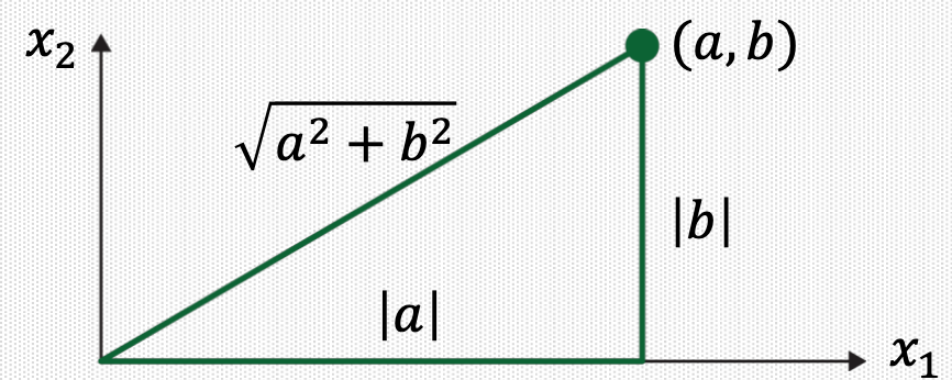
8. Geometric Meaning of Vector Norm
Suppose \(\mathbf{v} \in \mathbb{R}^{2}\), say, \(\mathbf{v}=\left[\begin{array}{l}a \\ b\end{array}\right]\).
\(\|\mathbf{v}\|\) is the length of the line segment from the origin to \(\mathbf{v}\).
This follows from Pythagorean Theorem applied to a triangle such as the one shown in the following figure:
For any scalar \(c\), the length \(c \mathbf{v}\) is \(|c|\) times the length of \(\mathbf{v}\), that is, \(\|c \mathbf{v}\|=|c|\|\mathbf{v}\|\).
9. Unit Vector
A vector whose length is \(1\) is called a unit vector.
Normalizing a vector: Given a nonzero vector \(\mathbf{v}\), if we divide it by its length, we obtain a unit vector \(\mathbf{u}=\frac{1}{\|\mathbf{v}\|} \mathbf{v}\).
\(\mathbf{u}\) is in the same direction as \(\mathbf{v}\), but its length is \(1\).
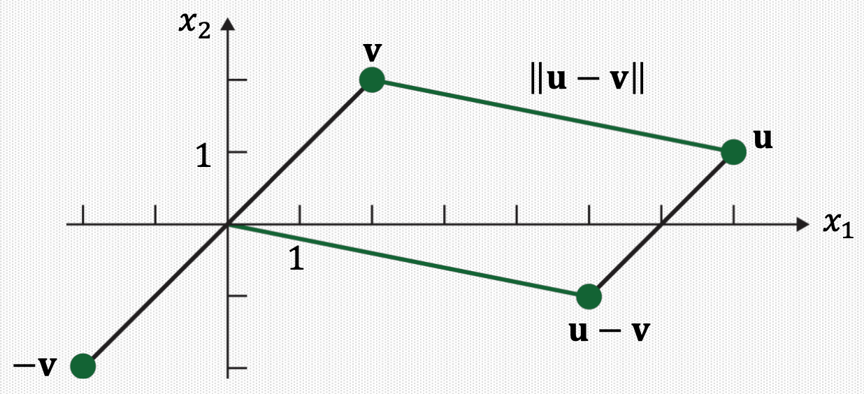
10. Distance between Vectors in \(\mathbb{R}^{n}\)
Definition: For \(\mathbf{u}\) and \(\mathbf{v}\) in \(\mathbb{R}^{n}\), the distance between \(\mathbf{u}\) and \(\mathbf{v}\), written as dist \((\mathbf{u}, \mathbf{v})\), is the length of the vector \(\mathbf{u}-\mathbf{v}\), that is, dist \((\mathbf{u}, \mathbf{v})=\|\mathbf{u}-\mathbf{v}\|\).
Example
The distance from \(\mathbf{u}\) to \(\mathbf{v}\) is the same as the distance from \(\mathbf{u}-\mathbf{v}\) to \(0\).
11. Inner Product and Angle Between Vectors
Inner product between \(\mathbf{u}\) and \(\mathbf{v}\) can be rewritten using their norms and angle:
Example

12. Orthogonal Vectors
Definition: \(\mathbf{u} \in \mathbb{R}^{n}\) and \(\mathbf{v} \in \mathbb{R}^{n}\) are orthogonal (to each other) if \(\mathbf{u} \cdot \mathbf{v}=0\), that is, \(\mathbf{u} \cdot \mathbf{v}=\|\mathbf{u}\|\|\mathbf{v}\| \cos \theta=0\).
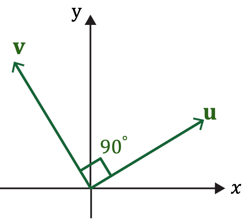
→ \(\mathbf{u} \cdot \mathbf{v} {c o s} \theta=0\) for nonzero vectors \(\mathbf{u}\) and \(\mathbf{v}\)
→ \(\theta=90^{\circ}(\mathbf{u} \perp \mathbf{v})\)
→ \(\mathbf{u}\) and \(\mathbf{v}\) are perpendicular each other.
13. Back to Over-Determined System
Let's start with the original problem:
Using the inverse matrix, the solution is \(\mathbf{x}=\left[\begin{array}{c}-0.4 \\ 20 \\ -20\end{array}\right]\)
Let's add one more example:
Now, let's use the previous solution \(\mathbf{x}={\left[\begin{array}{c}-0.4 \\ 20 \\ -20\end{array}\right]}\)
\(\left[\begin{array}{ccc}60 & 5.5 & 1 \\65 & 5.0 & 0 \\55 & 6.0 & 1 \\50 & 5.0 & 1\end{array}\right]{\left[\begin{array}{c}-0.4 \\20 \\-20\end{array}\right]}=\left[\begin{array}{l}66 \\74 \\78 \\{60}\end{array}\right] \neq\left[\begin{array}{l}66 \\74 \\78 \\{72}\end{array}\right] \quad \begin{gathered}\text { Errors } \\0 \\0 \\0 \\{12}\end{gathered}\)
How about using slightly different solution \(\mathbf{x}={\left[\begin{array}{c}-0.12 \\16 \\-9.5\end{array}\right]}\)?
\(\left[\begin{array}{ccc}60 & 5.5 & 1 \\65 & 5.0 & 0 \\55 & 6.0 & 1 \\50 & 5.0 & 1\end{array}\right]{\left[\begin{array}{c}-0.12 \\16 \\-9.5\end{array}\right]}=\left[\begin{array}{l}{71.3} \\{72.2} \\{79.9} \\{64.5}\end{array}\right] \neq\left[\begin{array}{l}{66} \\{74} \\{78} \\{72}\end{array}\right] \quad \begin{gathered}\text { Errors } \\{-5.3} \\{1.8} \\{-1.9} \\{7.5}\end{gathered}\)
14. Which One is Better Solution?
\(\left[\begin{array}{ccc}60 & 5.5 & 1 \\65 & 5.0 & 0 \\55 & 6.0 & 1 \\50 & 5.0 & 1\end{array}\right]{\left[\begin{array}{c}-0.12 \\16 \\-9.5\end{array}\right]}=\left[\begin{array}{l}{71.3} \\{72.2} \\{79.9} \\{64.5}\end{array}\right] \neq\left[\begin{array}{l}{66} \\{74} \\{78} \\{72}\end{array}\right] \quad \begin{gathered}\text { Errors } \\{-5.3} \\{1.8} \\{-1.9} \\{7.5}\end{gathered}\)\(\left[\begin{array}{ccc}60 & 5.5 & 1 \\65 & 5.0 & 0 \\55 & 6.0 & 1 \\50 & 5.0 & 1\end{array}\right]{\left[\begin{array}{c}-0.4 \\20 \\-20\end{array}\right]}\ \ =\left[\begin{array}{l}66 \\74 \\78 \\{60}\end{array}\right] \neq\left[\begin{array}{l}66 \\74 \\78 \\{72}\end{array}\right] \quad \begin{gathered}\ \ \ \text { Errors } \\0 \\0 \\0 \\{12}\end{gathered}\)
15. Least Squares: Best Approximation Criterion
Let's use the squared sum of errors:
\(\left[\begin{array}{ccc}60 & 5.5 & 1 \\65 & 5.0 & 0 \\55 & 6.0 & 1 \\50 & 5.0 & 1\end{array}\right]{\left[\begin{array}{c}-0.12 \\16 \\-9.5\end{array}\right]}=\left[\begin{array}{l}{71.3} \\{72.2} \\{79.9} \\{64.5}\end{array}\right] \neq\left[\begin{array}{l}{66} \\{74} \\{78} \\{72}\end{array}\right] \begin{gathered}\text { Errors } \\{-5.3} \\{1.8} \\{-1.9} \\{7.5}\end{gathered}\begin{gathered}\text{Sum of squared errors}\\\left({(-5.3)^{2}+1.8^{2}+(-1.9)^{2}+7.5^{2}}\right)^{0.5} \\=9.55\end{gathered}\)
\(\left[\begin{array}{ccc}60 & 5.5 & 1 \\65 & 5.0 & 0 \\55 & 6.0 & 1 \\50 & 5.0 & 1\end{array}\right]{\left[\begin{array}{c}-0.4 \\20 \\-20\end{array}\right]} =\left[\begin{array}{l}66 \\74 \\78 \\{60}\end{array}\right] \neq\left[\begin{array}{l}66 \\74 \\78 \\{72}\end{array}\right] \begin{gathered}\text { Errors } \\0 \\0 \\0 \\{12}\end{gathered}\begin{gathered}\text{Sum of squared errors}\\\left(0^{2}+0^{2}+0^{2}+{(-12)^{2}}\right)^{0.5} \\=12\end{gathered}\)
16. Least Squares Problem
Now, the sum of squared errors can be represented as \(\|\mathbf{b}-A \mathbf{x}\|\).
Definition: Given an overdetermined system \(A \mathbf{x} \simeq \mathbf{b}\) where \(A \in \mathbb{R}^{m \times n}\), \(\mathbf{b} \in \mathbb{R}^{n}\), and \(m \gg n\), a least squares solution \(\hat{\mathbf{x}}\) is defined as \(\widehat{\mathbf{x}}=\arg \min _{\mathbf{x}}\|\mathbf{b}-A \mathbf{x}\|\)
The most important aspect of the least squares problem is that no matter what \(\mathbf{x}\) we select, the vector \(A \mathbf{x}\) will necessarily be in the column space \(\operatorname{Col}A\).
Thus, we seek for \(\mathbf{x}\) that makes \(A \mathbf{x}\) as the closest point in \(\operatorname{Col}A\) to \(\mathbf{b}\).