6. Linear Transformation

1. 키워드

Linear Transformation(선형변환): 선형결합을 보존하는, 두 벡터 공간 사이의 함수

2. Transformation

A transformation, function or mapping, \(T\) maps an input \(x\) to an output \(y\)

Mathematical notaion: \(T: x \mapsto y\)

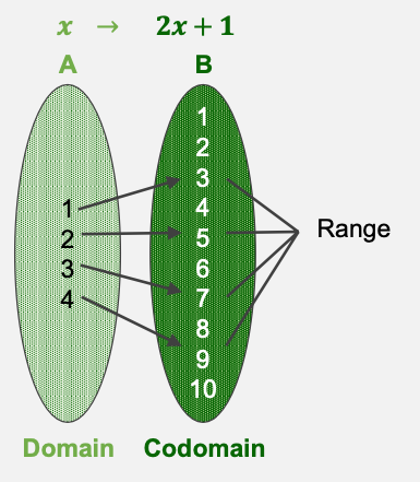
Domain(정의역): Set of all the possible values of \(x\)

Co-domain(공역): Set of all the possible values of \(y\)

Image: a mapped output \(y\), given \(x\)

Range(치역): Set of all the output values mapped by each \(x\) in the domain

Note that the output mapped by a particular \(x\) is uniquely determined.

3. Linear Transformation

Definition: A transformation (or mapping) \(T\) is linear if:

\(T(c \mathbf{u}+d \mathbf{v})=c T(\mathbf{u})+d T(\mathbf{v})\) for all \(\mathbf{u}\), \(\mathbf{v}\) in the domain of \(T\) and for all scalars \(c\) and \(d\)

Simple example: \(T: x \mapsto y\), \(T(x)=y=3 x\)

4. Transformations between Vectors

\(T: \mathbf{x} \in \mathbb{R}^{n} \mapsto \mathrm{y} \in \mathbb{R}^{m}\): Mapping \(n\)-dim vector to \(m\)-dim vector

Example

\[ T: \mathbf{x} \in \mathbb{R}^{3} \mapsto \mathbf{y} \in \mathbb{R}^{2} \quad \mathbf{x}=\left[\begin{array}{l}1 \\2 \\3\end{array}\right] \in \mathbb{R}^{3} \quad \mapsto \quad \mathrm{y}=T(\mathbf{x})=\left[\begin{array}{l}4 \\5\end{array}\right] \in \mathbb{R}^{2} \]

5. Matrix of Linear Transformation

Suppose \(T\) is a linear transformation from \(\mathbb{R}^{2}\) to \(\mathbb{R}^{3}\) such that:

\(T\left(\left[\begin{array}{l}1 \\ 0\end{array}\right]\right)=\left[\begin{array}{c}2 \\ -1 \\ 1\end{array}\right]\) and \(T\left(\left[\begin{array}{l}0 \\ 1\end{array}\right]\right)=\left[\begin{array}{l}0 \\ 1 \\ 2\end{array}\right]\). With no additional information, find a formula for the image of an aribitrary \(\mathbf{x}\) in \(\mathbb{R}^{2}\).

\(\begin{aligned}& \mathbf{x}=\left[\begin{array}{l}x_{1} \\x_{2}\end{array}\right]=x_{1}\left[\begin{array}{l}1 \\0\end{array}\right]+x_{2}\left[\begin{array}{l}0 \\1\end{array}\right] \\& \ \ \ \Rightarrow T(\mathbf{x})=T\left(x_{1}\left[\begin{array}{l}1 \\0\end{array}\right]+x_{2}\left[\begin{array}{l}0 \\1\end{array}\right]\right)=x_{1} T\left(\left[\begin{array}{l}1 \\0\end{array}\right]\right)+x_{2} T\left(\left[\begin{array}{l}0 \\1\end{array}\right]\right) \\& \qquad \qquad \ \ =x_{1}\left[\begin{array}{c}2 \\-1 \\1\end{array}\right]+x_{2}\left[\begin{array}{l}0 \\1 \\2\end{array}\right]=\left[\begin{array}{cc}2 & 0 \\-1 & 1 \\1 & 2\end{array}\right]\left[\begin{array}{l}x_{1} \\x_{2}\end{array}\right] \end{aligned}\)

In general, let \(T: \mathbb{R}^{n} \rightarrow \mathbb{R}^{m}\) be a linear transformation. Then \(T\) is always written as a matrix-vector multiplication, i.e., \(T(\mathbf{x})=A \mathbf{x}\) for all \(\mathbf{x} \in \mathbb{R}^{n}\)

In fact, the \(j\)-th column of \(A \in \mathbb{R}^{m \times n}\) is equal to the vector \(T\left(\mathbf{e}_{j}\right)\), where \(\mathbf{e}_{j}\) is the \(j\)-th column of the identity matrix in \(\mathbb{R}^{n \times n}\):

\[ A=\left[\begin{array}{lll}T\left(\mathbf{e}_{1}\right) & \cdots & T\left(\mathbf{e}_{n}\right)\end{array}\right] \]

Here, the matrix \(A\) is called the standard matrix of the linear transformation \(T\).

Find the standard matrix \(A\) of a llinear transformation from \(\mathbb{R}^{3}\) to \(\mathbb{R}^{2}\) such that:

\(T\left(\left[\begin{array}{l}1 \\0 \\0\end{array}\right]\right)=\left[\begin{array}{l}1 \\2\end{array}\right]\), \(T\left(\left[\begin{array}{l}0 \\1 \\0\end{array}\right]\right)=\left[\begin{array}{l}4 \\3\end{array}\right]\), and \(T\left(\left[\begin{array}{l}0 \\0 \\1\end{array}\right]\right)=\left[\begin{array}{l}5 \\6\end{array}\right]\).

\(\begin{aligned}\mathbf{x} &=\left[\begin{array}{l}x_{1} \\x_{2} \\x_{3}\end{array}\right]=x_{1}\left[\begin{array}{l}1 \\0 \\0\end{array}\right]+x_{2}\left[\begin{array}{l}0 \\1 \\0\end{array}\right]+x_{3}\left[\begin{array}{l}0 \\0 \\1\end{array}\right] \\\Rightarrow T(\mathbf{x}) &=T\left(x_{1}\left[\begin{array}{l}1 \\0 \\0\end{array}\right]+x_{2}\left[\begin{array}{l}0 \\1 \\0\end{array}\right]+x_{3}\left[\begin{array}{l}0 \\0 \\1\end{array}\right]\right) \\&=x_{1} T\left(\left[\begin{array}{l}1 \\0 \\0\end{array}\right]\right)+x_{2} T\left(\left[\begin{array}{l}0 \\1 \\0\end{array}\right]\right)+x_{3} T\left(\left[\begin{array}{l}0 \\0 \\1\end{array}\right]\right) \\&=x_{1}\left[\begin{array}{l}1 \\2\end{array}\right]+x_{2}\left[\begin{array}{l}4 \\3\end{array}\right]+x_{2}\left[\begin{array}{l}5 \\6\end{array}\right]=\left[\begin{array}{lll}1 & 4 & 5 \\2 & 3 & 6\end{array}\right]\left[\begin{array}{l}x_{1} \\x_{2} \\x_{3}\end{array}\right]=A \mathbf{x}\end{aligned}\)